Situatie
Running totals show how figures build over an extended period, one entry at a time, allowing you to see trends and patterns that raw data alone might not reveal. Creating running totals in Excel is straightforward, but you must be careful to use the correct method depending on how your data is structured.
Solutie
Pasi de urmat
Creating Running Totals in Regular Ranges
To create a running total in an Excel range that isn’t formatted as an Excel table, you need to use a combination of absolute and relative references.
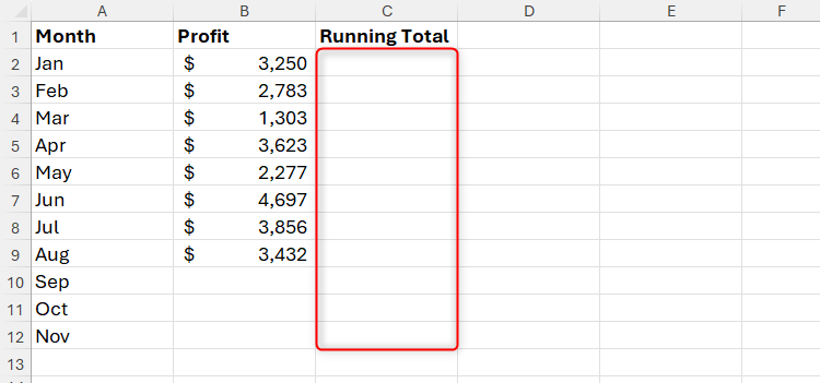
In this example, you want the Running Total column to update each time you add another value to the Profit column.
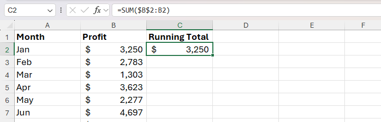
To do this, in cell C2, type:
=SUM($B$2:B2)
and press Ctrl+Enter to commit the formula and stay in the same cell.
Rather than typing the dollar symbols manually, place your cursor within the cell reference in the formula, and press F4.
Adding dollar symbols to the first reference (known as an absolute reference) fixes it. In other words, whenever the formula calculates the running total on each row, it will always take this cell as the start of the values to sum. On the other hand, the second reference doesn’t contain dollar symbols (known as a relative reference), because each time you duplicate the formula to the next row, you want it to pick up the corresponding figure.
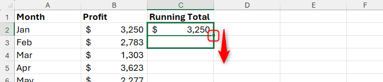
To see this in action, first, click and drag the fill handle in cell C2 down to cell C3.
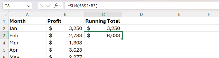
Then, select cell C3, and note that the formula in the formula bar is:
=SUM($B$2:B3)
The absolute $B$2 reference has remained fixed, while the relative B3 reference picks up the next value in the Profit column to update the running total.
You can now click and drag the fill handle to the bottom of the range so the formula is ready to pick up any new values you add to the subsequent rows.
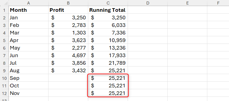
However, there’s one issue with this as it stands—the running total is repeated even in the rows where there aren’t yet any profit figures. While these totals are technically correct, they look untidy and could cause confusion.
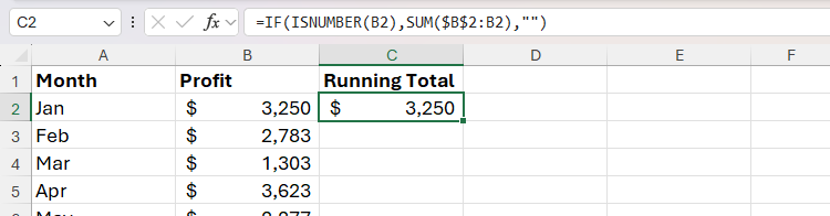
There are various ways to fix this, but my preferred method is to use the IF function. Here’s the formula to type into cell C2:
=IF(ISNUMBER(B2),SUM($B$2:B2),"")
In other words, if cell B2 contains a number, you want Excel to calculate the running total in cell C2 as in the example above. However, if cell B2 doesn’t contain a number, you want cell C2 to remain blank.
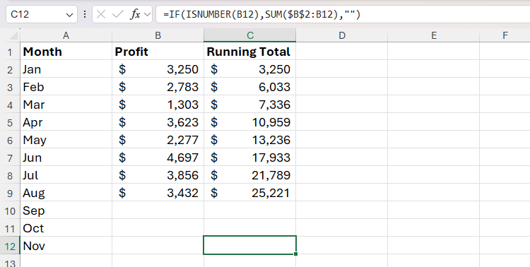
Now, when you click and drag the fill handle to the bottom of the range, only when there is a number in a cell in column B do you see the running total in the corresponding cell in column C.
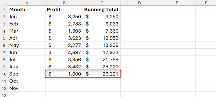
Click and drag the fill handle further down than the current bottom edge of the range to allow for potential growth. As you can see in the screenshot below, when I add a value to cell B10, the running total updates in cell C10.
If, like me, you prefer your data to be formatted as a structured Excel table, you’ll need to use a different method to create a running total. Specifically, there are two key differences between creating running totals in unformatted ranges and formatted tables.
First, rather than using cell references, you need to use structured references. This means that you can use the column headers in your table. Second, if you use the same formula as in regular ranges, Excel will struggle to correctly continue the running total if you add new rows to the bottom of your table.
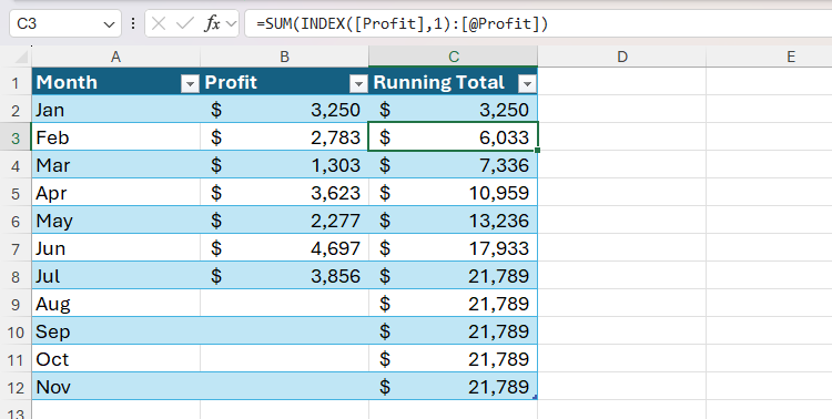
Instead, you need to use the INDEX function. In cell C2, type:
=SUM(INDEX([Profit],1):[@Profit])
where INDEX([Profit],1 tells Excel to start the calculation in the first row of the Profit column, and [@Profit] tells Excel that the final value to consider in the calculation is in the current relative row of the same column.
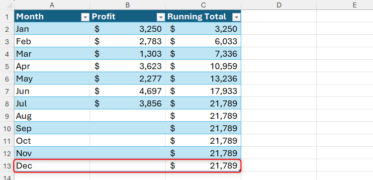
When you press Enter, the formula will automatically duplicate down the rest of column C.
What’s more, if you add a new row to the bottom of your table, the formula is automatically extended downwards.
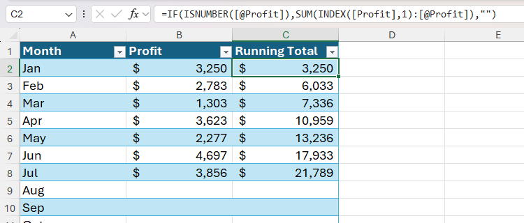
However, as with the previous example, the running total is repeated in the rows where there aren’t yet any profit figures, so you need to use the IF function to tell Excel to return a blank in any rows where there isn’t a value in the Profit column:
=IF(ISNUMBER([@Profit]),SUM(INDEX([Profit],1):[@Profit]),"")
Instead of using the INDEX function, you could use the TAKE function with exactly the same syntax. Whereas the INDEX function returns a value from a specified row or column from anywhere in an array, the TAKE function returns a specified number of rows or columns from the beginning or end of an array. However, unlike the TAKE function, the INDEX function is compatible with older versions of Excel.
PivotTables are a great way to summarize and manipulate your data for quick analysis, so adding a running total column is a great way to make your cumulative data even more useful.
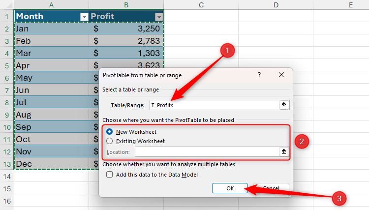
To create the PivotTable, select the cells containing the raw data, and in the Insert tab on the ribbon, click the top half of the “PivotTable” button.
Then, in the PivotTable From Table Or Range dialog box, double-check that the correct table or range is selected, decide whether you want the PivotTable to be placed on the same worksheet as the source data or a new worksheet, and click “OK.”
Having your PivotTable in a separate worksheet from the source data helps keep your Excel workbook more organized if you’re working with a particularly large dataset. Just remember to rename the new tab so you can easily tell what each worksheet contains.
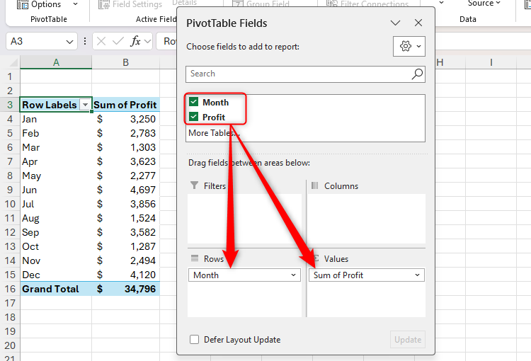
Now, click and drag the “Month” field into the Rows area of the PivotTable Fields pane, and the “Profit” field into the Values area.
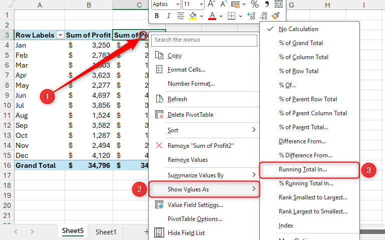
To create a running total of the Profit column, you first need to create a second column in the PivotTable containing the same data. So, click and drag “Profit” into the Values area again, exactly as you did in the previous step.

Next, right-click the column header of the second Profit column, hover over “Show Values As,” and click “Running Total In.”
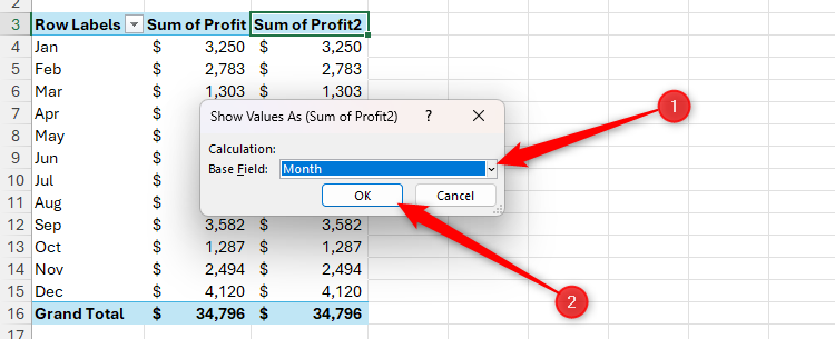
Then, choose an option in the Base Field drop-down menu, and click “OK”.
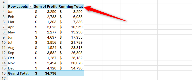
And there you have it—a running total column in your PivotTable. The final thing you need to do is change the column header to Running Total so that the PivotTable is easy to read.
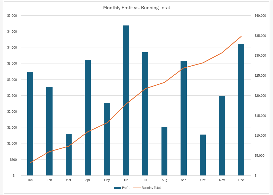
Once you’ve added your running total column, visualize your data as a chart to further emphasize its trends and patterns. To do this, select the column or columns you want to visualize, and in the Insert tab on the ribbon, click the relevant chart. Here, I created a combo chart that shows monthly totals as columns and the running total as a line. That way, I can compare the monthly data and monitor the bigger picture at the same time.
Leave A Comment?