Situatie
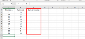
Start a new column anywhere in an Excel spreadsheet and label it. It’s here that we’ll output the solution of our squares. The squares don’t have to be next to each other, nor does the output section; it can be anywhere on the page.
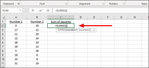
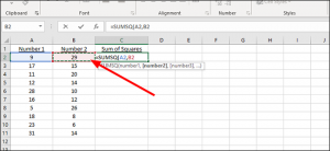
Type the following formula into the first cell in the new column: =SUMSQ(
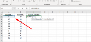
From here you can add the letter and number combination of the column and row manually, or just click it with the mouse. We’ll use the mouse, which autofills this section of the formula with cell A2.
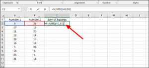
Add a comma and then we’ll add the next number, from B2 this time. Just type in B2 to the formula, or click the appropriate cell to autofill it.
Close the parenthesis and press “Enter” on the keyboard to display the sum of both squares. Alternatively, if you can keep going here, adding additional cells by separating each with a comma within the formula.
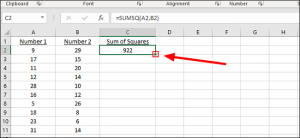
To apply the formula to additional cells, look for the small filled square in the cell that contains the solution to our first problem. In this example, it’s C2.
Click the square and drag it down to the last row of number pairs to automatically add the sum of the rest of the squares.
Finding the Sum of Squares for Just a Few Cells
In our “Sum of Squares” column we created in the previous example, C2 in this case, start typing the following formula:
=SUM((A2)^2,(A3)^2)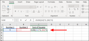
Alternatively, we can just add the numbers instead of the cells to the formula, as either way gets us to the same place.
That formula looks like this:
=SUM((9)^2, (29)^2)
You can alter these formulas as needed, changing the cells, adding additional numbers, or finding the sum of squares that aren’t even in your workbook, for example. And while it’s easier to follow along with the above tutorial, using the SUMSQ formula, to find the solution for multiple squares, it’s often easier to just type out a quick formula like this if it’s not something you’ll be repeating throughout the workbook.



Leave A Comment?