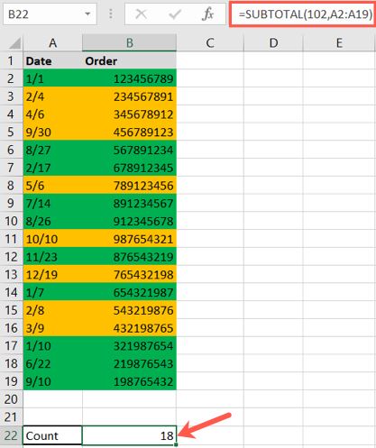
Go to the cell where you want to display your count. Enter the following, replacing the A2:A19 references with those for your own range of cells, and hit Enter.

=SUBTOTAL(102,A2:A19)

The number 102 in the formula is the numerical indicator for the COUNT function. As a quick check to make sure you entered the function correctly, you should see a count of all cells with data as the result.

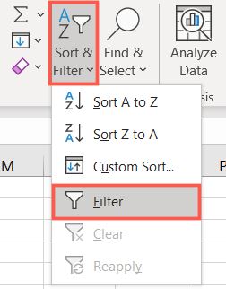
Now it’s time to apply the filter feature to your cells. Select your column header and go to the Home tab. Click “Sort & Filter” and choose “Filter”.

This places a filter button (arrow) next to each column header. Click the one for the column of colored cells you want to count and move your cursor to “Filter by Color.” You’ll see the colors you’re using in a pop-out menu, so click the color you want to count.

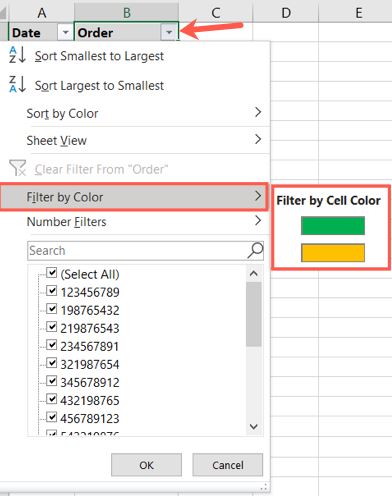
Note: If you use font color instead of or in addition to cell color, those options will display in the pop-out menu.

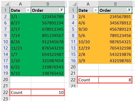
When you look at your subtotal cell, you should see the count change to only those cells for the color you selected. And you can pop right back up to the filter button and choose a different color in the pop-out menu to quickly see those counts too.

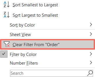
After you finish getting counts with the filter, you can clear it to see all of your data again. Click the filter button and choose “Clear Filter From”.

If you’re already taking advantage of colors in Microsoft Excel, those colors can come in handy for more than just making data stand out.