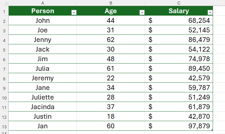
In this case, thinking back to the syntax above, column B contains the values you want to test (argument x), more than 40 is the criterion (argument y) for the values in column B, and column C contains the values you want to average (argument z).

So, in a separate cell, you need to type:

=AVERAGEIF(Table1[Age],">40",Table1[Salary])

and press Enter.

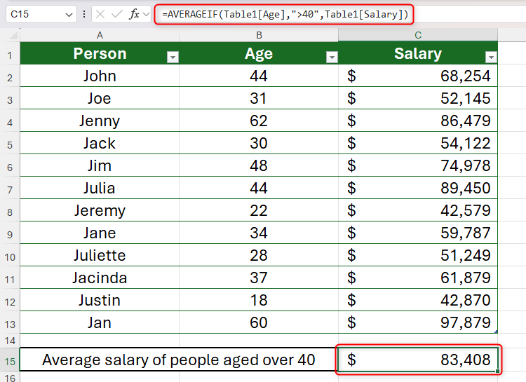
The first thing you’ll notice is the use of structured references for arguments x and z. In other words, rather than using direct cell references (such as B2:B13 for argument x and C2:C13 for argument z), the formula references the column headers. This is because the data is contained within a formatted Excel table, and the program defaults to using the table headers in formulas. This means that if you add extra rows to the bottom of your data, the formula will automatically include those new values.

Before you go ahead and use AVERAGEIF in your own spreadsheet, there are some important points you should be aware of.

First, argument y (the test) is very flexible. While the example above uses “>40” (a logical operator) to test the range in argument x, there are various other types of criteria you could use instead:

Second, the AVERAGEIF function doesn’t consider empty cells. For example, if someone’s salary value was blank, it would be ignored in the average calculation. However, if someone’s salary was $0, this would be included in the average calculation.

Finally, if none of the specified cells meets the test, Excel returns the #DIV/0! error to tell you that it can’t calculate the average. Where AVERAGEIF tests one condition before calculating the average of all values that meet the test, AVERAGEIFS allows you to narrow your results even further by using several criteria.

The AVERAGEIFS Syntax

It’s important to note that the order and number of arguments in the AVERAGEIFS function differs significantly from the AVERAGEIF function:

=AVERAGEIFS(x,y¹,y²,z¹,z²,...)

where

• x (required) is the range of cells containing the values to be averaged,
• y¹ (required) is the range of cells containing the first values to be tested,
• y² (required) is the test for y¹,
• z¹ (optional) is the range of cells containing the second values to be tested, and
• z² (required if z¹ is included) is the test for z¹.

In other words, the syntax above represents the AVERAGEIFS function being used to create two tests (y and z), though you can include up to 127 tests overall.

AVERAGEIFS in Action

If the AVERAGEIFS syntax confuses you, things will become much clearer when you see how the function works in an example.

This Excel table contains people’s names, ages, genders, and salaries, and your aim is to work out the average salary of all males over the age of 35.

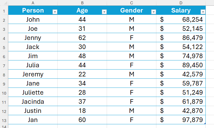
Since there are two criteria (age and gender), you need to use the AVERAGEIFS function:

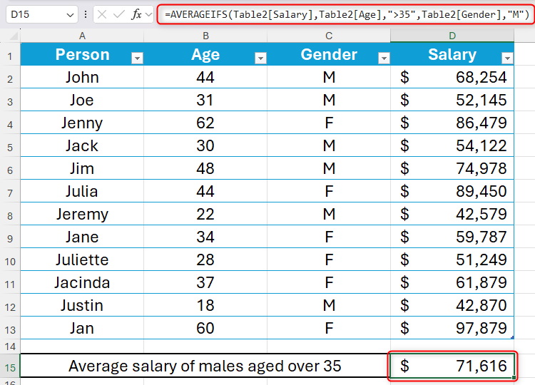
=AVERAGEIFS(Table2[Salary],Table2[Age],">35",Table2[Gender],"M")

where

• Table2[Salary] is the range of cells containing the values to be averaged (argument x),
• Table2[Age] is the range of cells containing the first set of values to be tested (argument y¹),
• “>35” is the test for the first range (argument y²),
• Table2[Gender] is the range of cells containing the second set of values to be tested (argument z¹), and
• “M” is the test for the second range (argument z²).

Here are some things to remember when using the AVERAGEIFS function:

• The tests can be logical arguments, values, text, cell references, or a combination of these.
• Logical arguments and text must always be enclosed in double quotations.
• Only cells that meet all conditions will be included in the average calculation.
• All ranges specified in an AVERAGEIFS formula must be the same size.
• The AVERAGEIFS function discounts empty cells but includes cells with a value of zero.
• The #DIV/0! error will be returned if no cells meet all the criteria.