The TRIMRANGE function has three arguments:

=TRIMRANGE(a,b,c)

where

• a (required) is the range to be trimmed,
• b (optional) determines which rows to trim (0 = no rows, 1 = leading rows, 2 = trailing rows, and 3 = both leading and trailing rows), and
• c (optional) determines which columns to trim (0 = no columns, 1 = leading columns, 2 = trailing columns, and 3 = both leading and trailing columns).

If you omit arguments b and/or c, Excel will default to trimming both the leading and trailing rows and/or columns.

At the time of writing (January 2025), TRIMRANGE doesn’t allow you to trim blank rows or columns between existing data. You can only use it to trim data before or after your data. Instead, use other ways to delete empty rows of data between populated rows of data.

Example 1: TRIMRANGE with a Sum

In this example, I want to subtract the values in column B from those in column C to produce a profit.

I know that I will add additional rows at the bottom at some point in the future, so I want Excel to automatically pick these up as part of the subtraction formula. To do this, I could type:

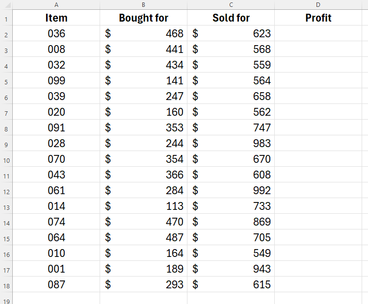
=(C2:C200)-(B2:B200)

into cell D2, as this would spill the references to the first 200 rows. However, doing this would result in an untidy spreadsheet with lots of empty calculations. What’s more, if I used whole-column references, the calculation would spill to the very bottom of the spreadsheet. This would cause there to be over a million calculations, thus significantly increasing my spreadsheet’s size and slowing it down.

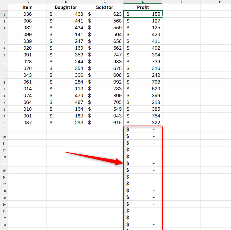
Instead, I will type:

=TRIMRANGE(C2:C200)-TRIMRANGE(B2:B200)

into cell D2, which would effectively trim the redundant cells at the bottom of my data to prevent Excel from having to work too hard and keep my spreadsheet looking tidy.

I’ve omitted arguments b and c in the above TRIMRANGE references, as Excel’s default of trimming leading and trailing columns and rows works well in this example, since there are no leading blank rows or columns, and there is no data to the right of column D.

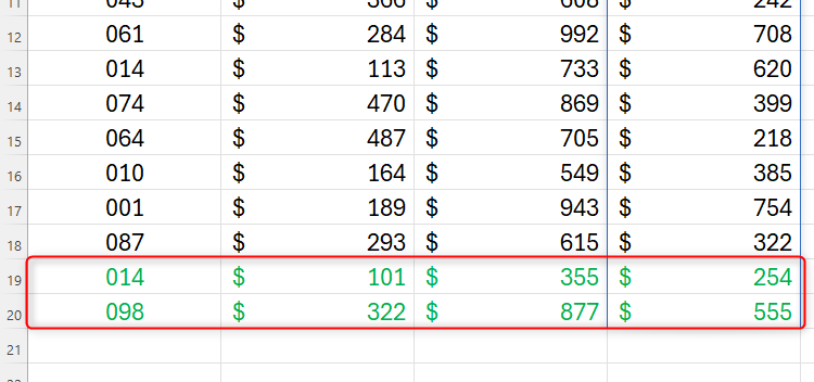
Now, when I add further rows of data at the bottom, the corresponding cells in the Profit column will calculate automatically.

Example 2: TRIMRANGE With XLOOKUP

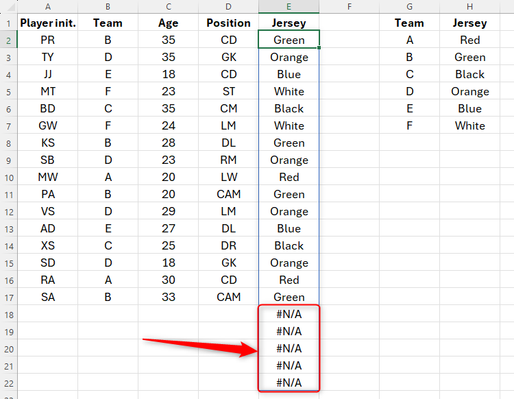
In this second example, I have a list of soccer players, and I’m going to use the XLOOKUP function to tell me which color jersey I need to provide them with, depending on the team they’re in.

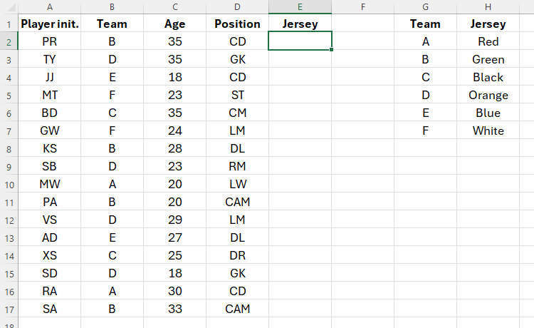
I also know that I’m going to recruit a further five players, so when I add my XLOOKUP formula, I need to extend it to row 22. So, in cell E2, I could type:

=XLOOKUP(B2:B22,$G$2:$G$7,$H$2:$H$7) where B2:B22 is the range, $G$2:$G$7 is the lookup array, and $H$2:$H$7 is the return array.
I’ve used $ symbols to tell Excel that these are absolute (fixed) cell references. However,
as with the previous example, this would leave the five rows of empty data looking untidy due to the #N/A error.Also, Excel is working harder than it needs to, an issue that could affect performance if you have lots of blank rows included in your formula.

I could also use OFFSET, INDEX, or TOCOL to create dynamic range formulas, but these are much more complicated ways to achieve the same outcome as the much simpler TRIMRANGE method.

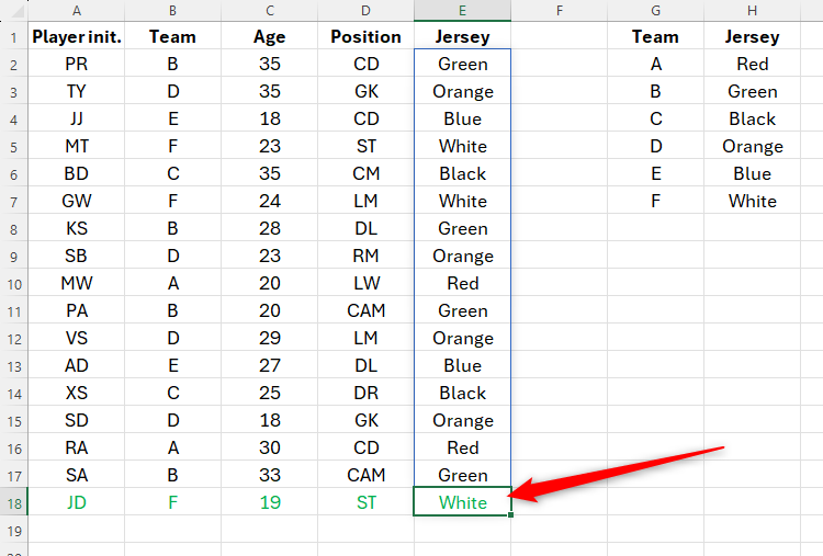
So, in cell E2, I will type:

=XLOOKUP(TRIMRANGE(B2:B22,2),$G$2:$G$7,$H$2:$H$7)

which is exactly the same formula as above, except that I’ve referenced the range (B2:B22) within the TRIMRANGE function. Notice how, this time, I’ve decided to include the second argument (“2”), which tells Excel that I want to trim trailing blank rows. However, I’ve not included a third argument, as my range only spans one column.

This time, Excel has trimmed my XLOOKUP result, and when I add more rows of data at the bottom, the cell in column E populates automatically.