Array Constants in Excel: Definition

An array constant is a hard-coded set of static values entered into a formula, enclosed in curly braces. In a straightforward example, typing:

={10,20,30,40}

into cell A1 and pressing Enter returns a dynamic array of 10 in cell A1, 20 in cell B1, 30 in cell C1, and 40 in cell D1.

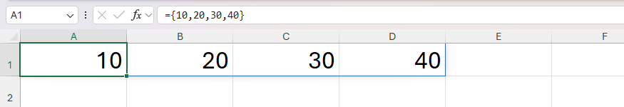
In the example above, the dynamic array result is spilled horizontally (in columns) because commas are used between each value in the array constant.

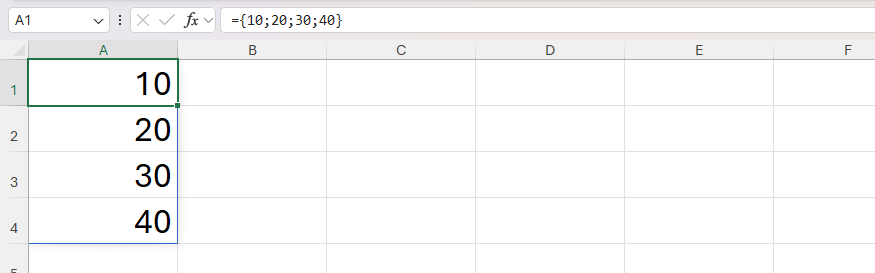
On the other hand, using semicolons between the values in the array constant returns a vertical dynamic array (in rows):

={10;20;30;40}

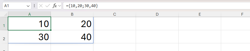
You can also combine commas and semicolons in an array constant to return a two-dimensional dynamic array:

={10,20;30,40}

Array Constants Work Differently Than They Used To

One-off versions of Excel from 2021 onward, Excel for Microsoft 365, and Excel for the web all support dynamic array formulas. This means that when you type an array constant in a formula that expects multiple values and press Enter, the result spills into the adjacent cells, with only the top-left cell containing a formula.

However, in older versions of Excel that don’t support dynamic array formulas, you need to select all the cells where you want the results to be displayed, type the formula, and press Ctrl+Shift+Enter to commit it. At this point, the same formula appears in all the cells you selected. This is known as a CSE or legacy array formula.

Using Array Constants With Excel Functions

Array constants are most useful in Excel when paired with functions, as they save you from having to input multiple or lengthy formulas. Here are two example scenarios.

SUM and COUNTIF: Counting How Many Values in an Array Meet Multiple Criteria

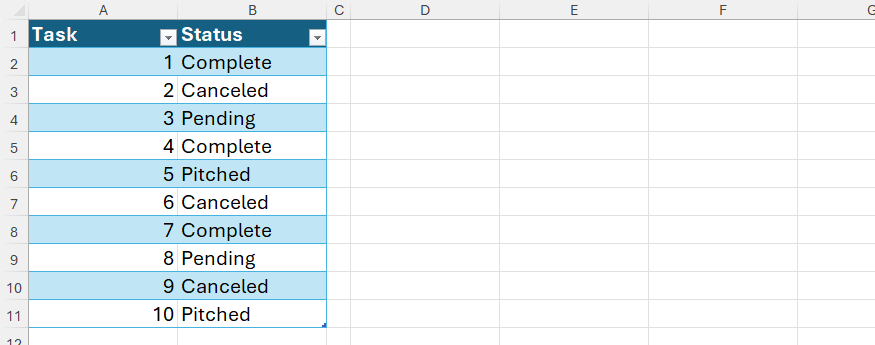
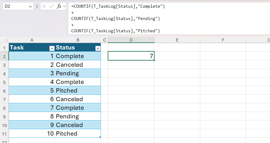
Imagine you have this Excel table, named T_TaskLog, and you want to find out the number of tasks whose status is Complete, Pending, or Pitched.

To do this without array constants, you might type the following formula (divided onto separate lines for easier reading):

=COUNTIF(T_TaskLog[Status],”Complete”)
+
COUNTIF(T_TaskLog[Status],”Pending”)
+
COUNTIF(T_TaskLog[Status],”Pitched”)

where the results of three separate COUNTIF formulas are added together using the plus (+) operator.

However, this formula is lengthy and difficult to parse. Instead, you can use array constants to group all the criteria into one argument. First, type the function’s name, an opening parenthesis, and the range to evaluate, followed by a comma:

=COUNTIF(T_TaskLog[Status],

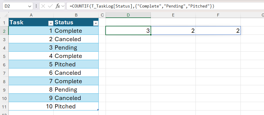
Now, for the criteria, you need to enter all three status values as an array constant, enclosed in curly braces. Then, add a closing parenthesis, and press Enter:

=COUNTIF(T_TaskLog[Status],{“Complete”,”Pending”,”Pitched”})

At this point, Excel returns three separate results as a dynamic array—3 for Complete, 2 for Pending, and 2 for Pitched. That’s because you haven’t yet told Excel to add the results together.

To fix this, wrap the whole formula inside the SUM function and press Enter:

=SUM(COUNTIF(T_TaskLog[Status],{“Complete”,”Pending”,”Pitched”}))

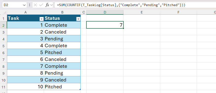
So, rather than using three separate COUNTIF formulas separated by the plus sign to count the three text criteria, the array constant forces Excel to perform the calculation three times—one for each criterion—and add the results together through the SUM function.

LARGE: Finding the Top x Values in a Range

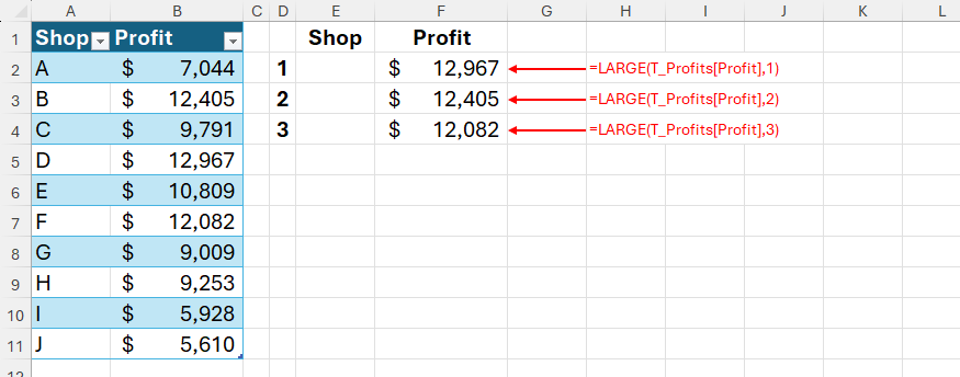
In this example, let’s say you want to return the top three profits from the table, named T_Profits, as a separate array.

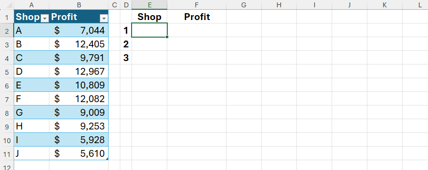
One way to do this is to use the LARGE function in three separate cells.

Typing this formula into cell E2 returns the largest value in the Profit column:

=LARGE(T_Profits[Profit],1)

Then, typing this formula into cell E3 returns the second largest value:

=LARGE(T_Profits[Profit],2

Finally, typing this formula into cell E4 returns the third largest value:

=LARGE(T_Profits[Profit],3)

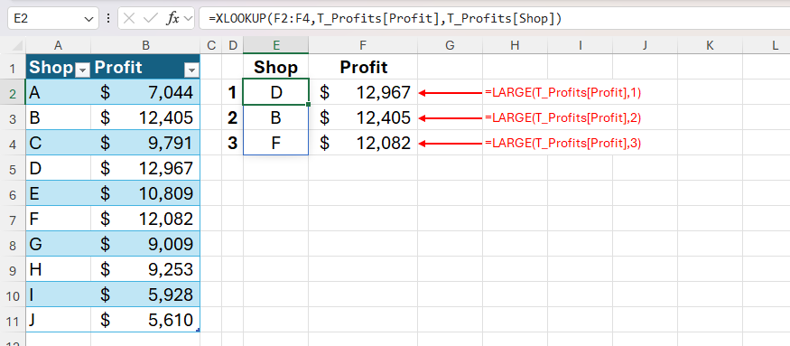
You can then use the XLOOKUP function to retrieve the IDs of the shops where these three highest profits were made:

=XLOOKUP(E2:E4,T_Profits[Profit],T_Profits[Shop])

However, typing three separate, unlinked formulas takes time and is prone to error. Instead, you can use an array constant with the LARGE function to achieve the same result with a single formula:

=LARGE(T_Profits[Profit],{1;2;3})

This formula applies the LARGE function three times—the first time to return the largest value, the second time to return the second largest value, and the third time to return the third largest value—and returns the three results as a vertical dynamic array because a semicolon is used between each number in the array constant.

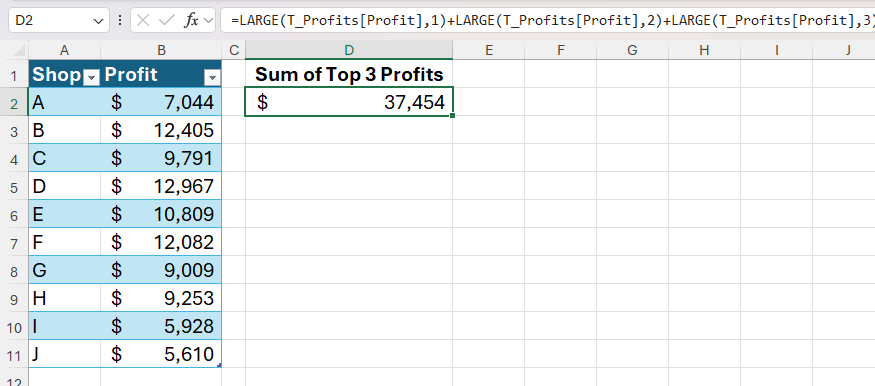
Similarly, if you want to sum the largest three profits without using array constants, you would need to input the LARGE function three times, separated by the plus sign:

=LARGE(T_Profits[Profit],1)+LARGE(T_Profits[Profit],2)+LARGE(T_Profits[Profit],3)

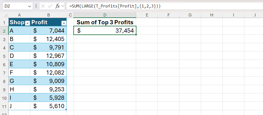
However, using an array constant with the SUM function makes the formula much tidier:

=SUM(LARGE(T_Profits[Profit],{1,2,3}))

What’s more, if you wanted to include the fourth largest profit in the calculation, you simply need to add a comma and the number four to the formula, rather than typing an extra LARGE function in its entirety:

=SUM(LARGE(T_Profits[Profit],{1,2,3,4}))

Naming Array Constants in Excel

If you find yourself repeatedly using the same set of static values in Excel, naming an array constant saves you from typing it manually each time.

To create a named array constant, in the Formulas tab on the ribbon, click “Name Manager.”

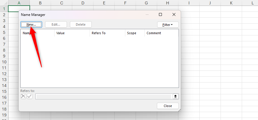
Then, in the Name Manager dialog box, click “New.”

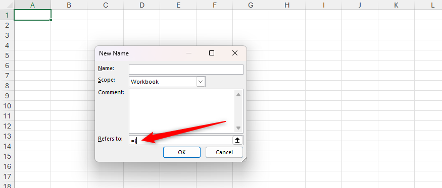
Next, in the Refers To field, type the equal sign, followed by an opening curly brace:

={

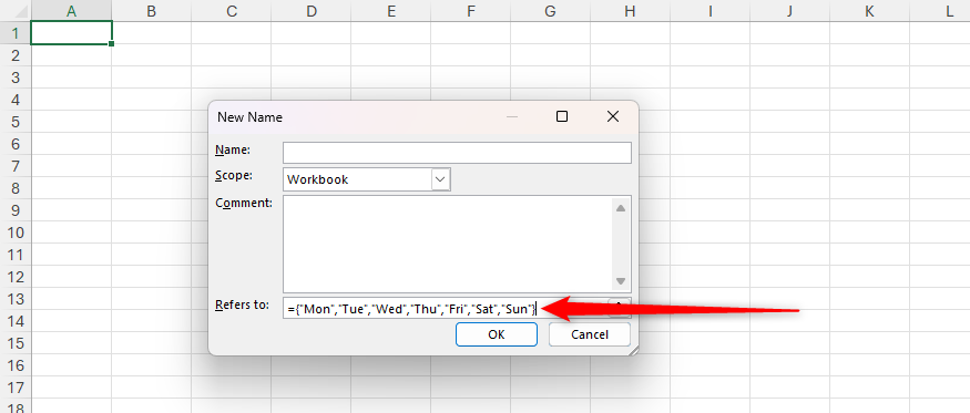
Now, type the array constant, remembering that to create a horizontal (row) array, the values must be separated by commas, and for vertical (column) arrays, you need to separate them with semicolons. Also, remember that text values must be enclosed in double quotes. When you’re done, close the curly braces:

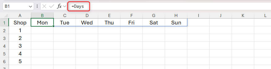
={“Mon”,”Tue”,”Wed”,”Thu”,”Fri”,”Sat”,”Sun”}

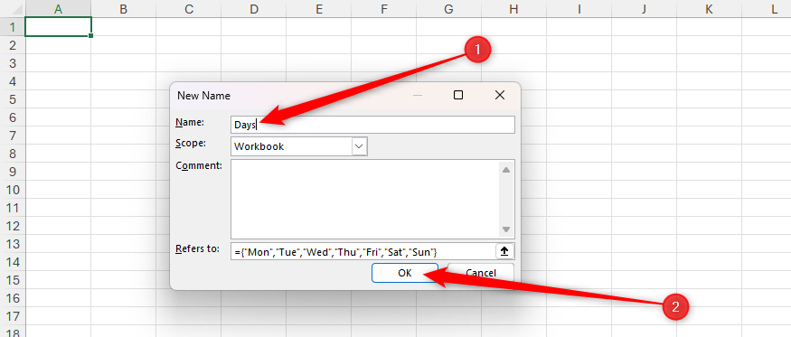
Finally, in the Name field, type a memorable name for your array constant, and click “OK”

You can now use this array constant in your workbook by typing the equal sign followed by the name you just assigned and pressing Enter:

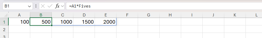
As with unnamed array constants, you can use them in formulas. In this example, the array constant named Fives is:

={5,10,15,20}

So, multiplying the value in cell A1 by this named array constant produces four separate results:

=A1*Fives

Points to Note When Using Array Constants in Excel

Despite the many benefits of using array constants in Excel, there are some rules and limitations you should be aware of:

• Dynamic array formulas cannot spill into structured table columns, so array constants that produce multi-cell results can only be used in regular cells. That said, array constants themselves can operate on data within tables.
• Array constants can only contain text in double quotes, plain numbers (no currency symbols or percent signs), or Boolean values (TRUE and FALSE), separated by the comma and semicolon delimiters. They can’t contain cell references, other arrays, formulas, or wildcards.
• Because you can’t reference cells in array constants, all values must be hard-coded (hence their name, array constants). As a result, formulas containing array constants are less flexible than those without.
• If you plan to share your workbook with people less experienced in Excel, beware of the black-box effect that array constants create. That is to say, because the calculation process in array constants is less transparent than in standard formulas, those unfamiliar with array logic might struggle to understand how the spreadsheet works.
• In some cases, using a dynamic array function is more efficient than using an array constant. For example, rather than inputting a constant such as {1,2,3}, you can use the SEQUENCE function to produce the same result.
• Because the way array constants are handled in Excel changed dramatically when dynamic arrays were introduced, when an Excel file created in a modern version is opened in an older version, spilled arrays are converted into CSE formulas.