Situatie
Generating random lists of numbers in Excel is handy for randomizing lists, statistical sampling, and many other uses. However, Excel’s random number functions are volatile, meaning they change constantly.
Solutie
Excel has three functions for generating random numbers:
| Function Name | What It Does | Syntax | Notes |
|---|---|---|---|
| RAND | Generates a random number between 0 and 1. | =RAND() | There are no arguments between the parentheses in this function’s formula. |
| RANDBETWEEN | Generates a random number between your specified minimum and maximum. | =RANDBETWEEN(a,b) | a is the bottom end of the range, and b is the top end of the range. |
| RANDARRAY | Generates an array of random numbers according to the criteria you set. | =RANDARRAY(v,w,x,y,z) | v is the number of rows to be returned, w is the number of columns to be returned, x is the bottom end of the range, y is the top end of the range, and z is TRUE if you want it to return whole numbers or FALSE if you want it to return decimal numbers. |
After typing your formula and pressing Enter, you can use Excel’s fill handle to create more random numbers using the same criteria. Do be careful, however, when using the fill handle with RANDARRAY—if you drag the fill handle to cells that would have contained the result for your initial RANDARRAY formula, you will see a #SPILL! error, and the array of random numbers will be interrupted.
How to fix the Random Numbers you Generated
All three of the random number functions listed above are volatile functions, meaning they regenerate each time a change is made to the worksheet or whenever the workbook is reopened.
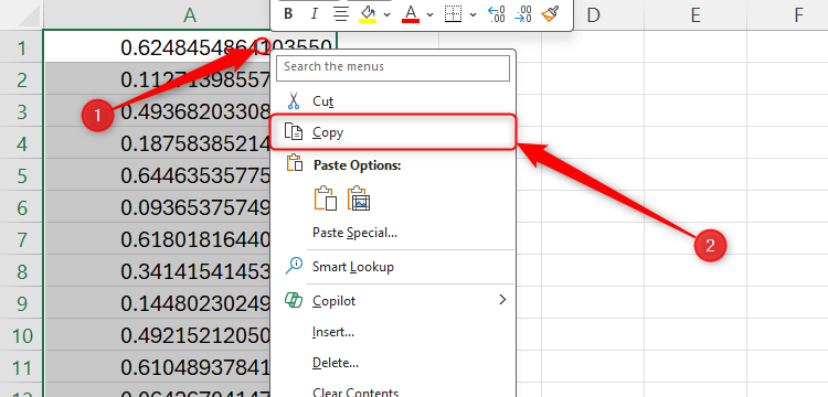
So, to fix the random numbers you generated (I used the RAND function in my example below), select the cells containing those numbers, right-click the selected cells, and click “Copy.” Alternatively, select the cells, and press Ctrl+C.
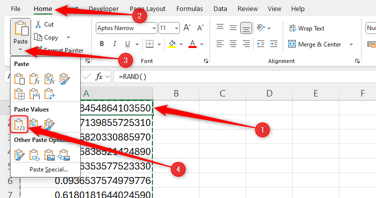
These numbers are now fixed as though you typed them into the cells manually. In essence, you used the random number function to create the numbers, and you then used Paste Special to fix them.
How to remove Duplicated Random Numbers
Before I show you how to remove duplicated values from your list of random numbers, it’s worth noting that the RAND function is the least likely of the three listed above to return any duplicates, as it produces a list of numbers containing up to 15 decimal places.
You can also increase the chances of avoiding repeated numbers when using the RANDARRAY function by typing FALSE as the final argument to return decimalized numbers.
However, since RANDBETWEEN uses integers (whole numbers only) and has upper and lower limits, whether it’s likely to return duplicates depends on the range you specify—the larger the range, the less likely the function is to return repeated numbers.
The steps below assume that you have fixed your random numbers (as discussed in the previous section). They also assume that all your random numbers are in one column.
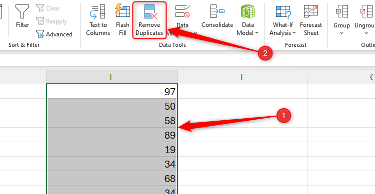
First, select all the cells containing the fixed random numbers. If you have a long list of numbers, it will be quicker to select the whole column instead. Then, in the Data tab, click “Remove Duplicates”.
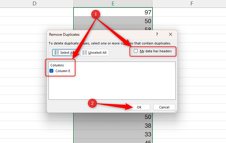
Next, make sure the details in the Remove Duplicates dialog box are correct. In my case, my data is in column E and doesn’t have headers, so I’m good to click “OK”.
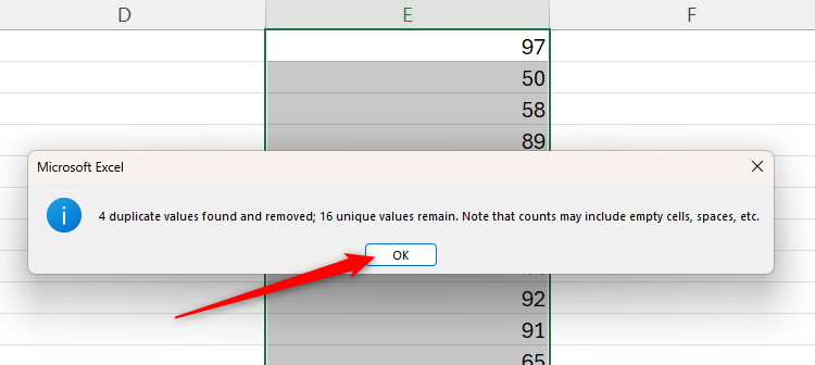
Excel then tells you how many duplicates it has removed. In my example, 50 appeared in the list three times, and 19 appeared twice, so Excel has removed two 50s and one 19, totaling four duplicate removals overall. Click “OK” to close this message.
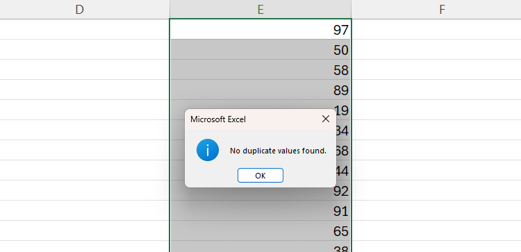
Now, because the data is four numbers light, I need to use the same random number function that I used in my original list to generate more random numbers, and fix them as I did in the previous step. When you’ve done the same, select the whole list of numbers again, click “Remove Duplicates” in the Data tab, and repeat the process until you no longer have any random numbers.
As well as copying and pasting the values in cells containing volatile functions to fix them, you can also stop all volatile functions from calculating automatically by clicking “Calculation Options” in the Formulas tab, and selecting “Manual.” Then, once you’ve entered your random number function, click “Calculate Now” to update the random values.
Leave A Comment?