The key to understanding how XLOOKUP can be used to perform two-way lookups is to first get your head around how this function works in one-dimensional scenarios.

The XLOOKUP function has six arguments:

=XLOOKUP(a,b,c,d,e,f)

where

• a (required) is the lookup value,
• b (required) is the lookup array,
• c (required) is the return array,
• d (optional) is the text to return if the lookup value (a) is not found in the lookup array (b),
• e (optional) is the match mode (0 = exact match; -1 = exact match or next smaller item; 1 = exact match or next larger item; 2 = wildcard match), and
• f (optional) is the search mode (1 = top to bottom or left to right; -1 bottom to top or right to left; 2 = binary search with the lookup array (b) in ascending order; -2 = binary search with the lookup array (b) in ascending order.

In this example, typing:

=XLOOKUP(F2,A2:A100,D2:D100,"Invalid ID",0,1)

into cell G2 returns a score of 48.

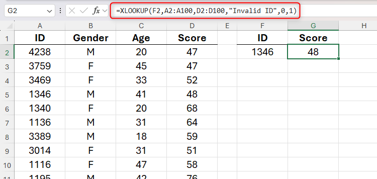
This formula takes the ID in cell F2 (argument a), looks for it in cells A2 to A100 (argument b), and returns the corresponding value in cells D2 to D100 (argument c). If the ID in cell F2 isn’t listed in cells A2 to A100, the lookup returns the term “Invalid ID” (argument d). The fifth argument tells Excel to return exact matches only (argument e), and the sixth ensures the lookup runs from the top of the range to the bottom of the range (argument f).

While one-way lookups are useful in many scenarios, they don’t allow you to change the variable you’re looking up. Indeed, the formula above only returns a score based on the specified ID, but what if you wanted to see the age or gender instead? This is where a two-way lookup (also known as a two-dimensional or matrix lookup) comes into play.

To do this, you need to nest one XLOOKUP inside the other:

=XLOOKUP(a¹,b¹,XLOOKUP(a²,b²,c))

where

• • a¹ and b¹ are the lookup value and array for the first variable,
  • a² and b² are the lookup value and array for the second variable, and
  • c is the return array.

Based on this, typing:

=XLOOKUP(F2,A2:A100,XLOOKUP(G1,B1:D1,B2:D100))

into cell G2 returns a score of 48.

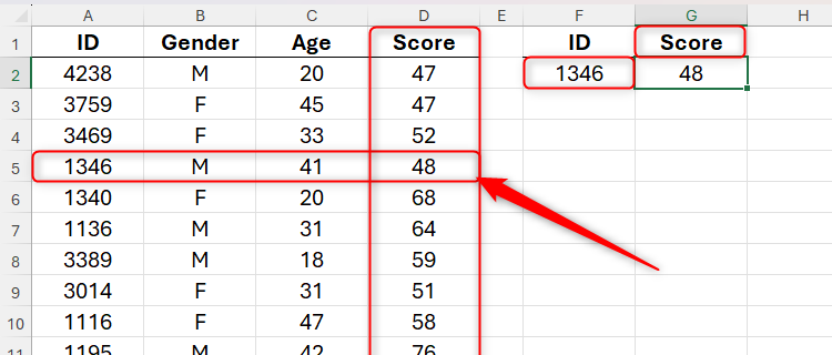
This is because Excel first searches for the specified ID (argument a¹) in cells A2 to A100 (argument b¹), then it searches for the specified variable (argument a²) in cells B1 to D1 (argument b²), and returns the result at the intersection of these two lookups in cells B2 to D100 (argument c).

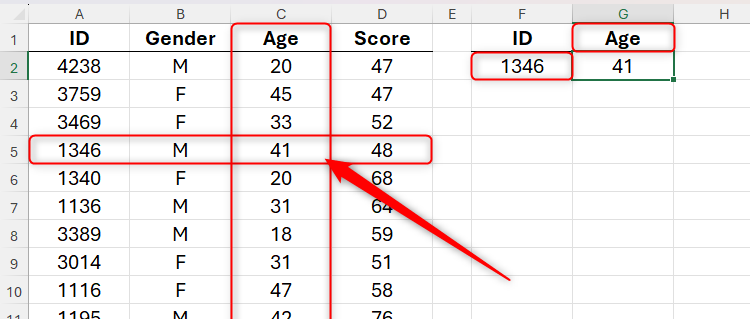
As a result, if you change the variable in cell G1 to “Age,” you get a result of 41.

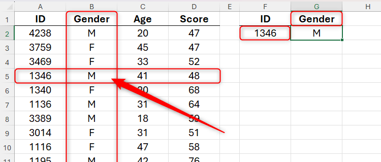
Likewise, if you change it to “Gender,” you get M as the result.

Pro Tip: Add Drop-Down Lists to the Lookup Cells

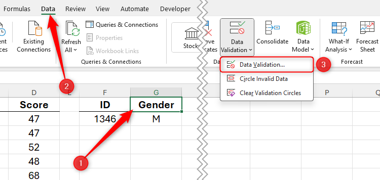
Now that your two-way lookup is complete, you could go one step further by adding a drop-down list to the cells containing the lookup values to speed up the data retrieval process. To do this, select one of the lookup cells (in this case, cell G1), and in the Data tab on the ribbon, click “Data Validation”.

Next, in the Allow field of the Data Validation dialog box, select “List.” Finally, activate the “Source” field, and select the cells containing the values that you want to appear in the drop-down list. In this case, it’s the column headers in cells B1 to D1.

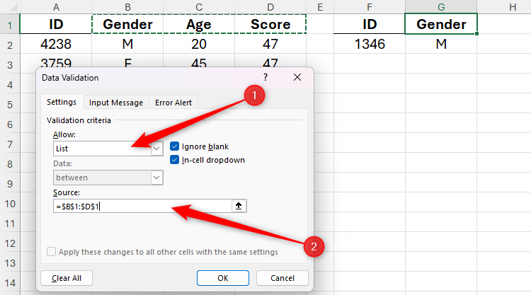
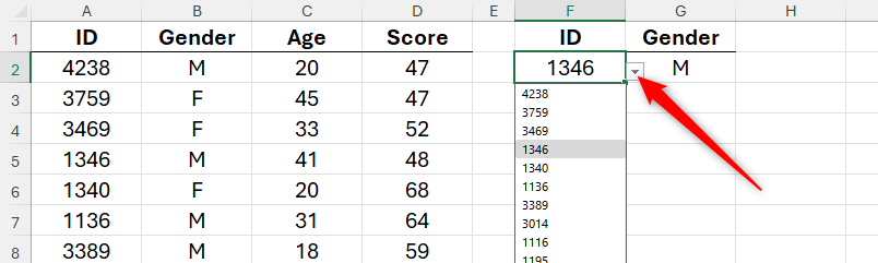
When you click “OK,” you’ll see a drop-down button in cell G1 which, when clicked, reveals the variable options.

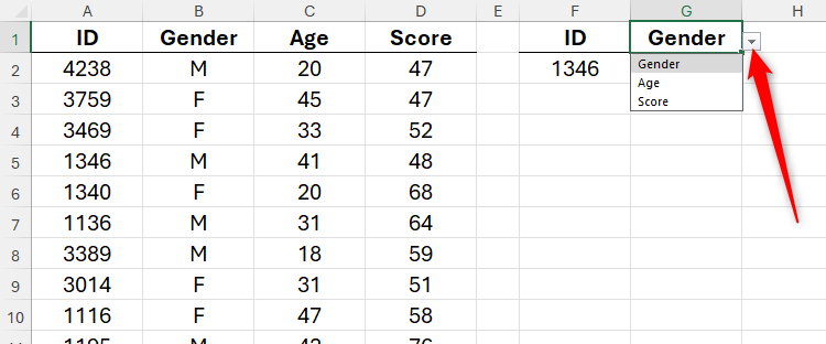
Now, repeat the process for cell F2, the other lookup cell.

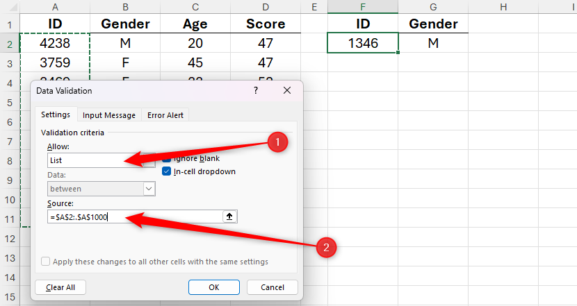
Notice how, in the Source field, I’ve specified a range that extends beyond the size of my dataset to allow for growth (my dataset contains 100 rows, but I’ve extended the source to cell A1000). The period (also known as a trim ref operator in this context) after the colon tells Excel to trim any blank cells at the end of the source range.

Alternatively, you could use a formula that counts the number of cells containing values in column A and returns that number of options in the drop-down menu. Now, you can select an ID from the drop-down list in cell F2.