Navigating multiple tabs is frustrating

The more Excel worksheets you have, the longer it takes to find the data you need.

The user interface for navigating worksheets is very clunky. Indeed, you can’t use the mouse scroll wheel to quickly jump between the sheets—you have to click the tiny navigation arrows repeatedly. Even if you maximize the tab area, Excel only allows you to view a handful of tabs at once, diverting your attention from your data and breaking your concentration and workflow. The fastest way to navigate between sheets is Ctrl+PgDn and Ctrl+PgUp, but this still forces you to cycle through many sheets.

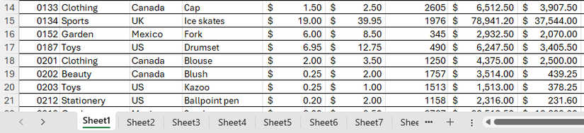
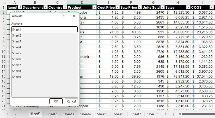
One workaround is to right-click the navigation arrows to bring up a vertical list of tabs. However, the physical friction of right-clicking, waiting for the dialog box, finding and selecting the right sheet, and clicking “OK” adds up, taking significantly more time and effort than finding the right row in a single-sheet dataset. What’s more, the index list that pops up covers cells on the current worksheet, potentially obscuring data you want to see.

Too many worksheets inflate file size

Every extra worksheet you add to your Excel workbook adversely affects overall performance.

This increase in file size isn’t just about raw data volume—it’s also due to hidden bloat from duplicated features, such as repeated headers and unnecessary formatting across multiple sheets. This collective weight significantly slows your entire spreadsheet operation, potentially making the file sluggish or even crash entirely when opening, saving, or performing complex calculations.

By consolidating your data into a single, structured Excel table (created by pressing Ctrl+T), you get rid of this bloat and simplify your workbook’s data model.

3D referencing is fragile

If you have like-for-like data on multiple tabs—like monthly sales figures—you’re likely to use 3D referencing, which is where you reference the same cell in several worksheets in a formula.

Useful as this might be, small changes can make the formula return incorrect results. One major risk is silent volatility. If a sheet is inserted or deleted within the defined range, the formula adjusts to the new range but doesn’t throw up an error, which can make the output unreliable. Similarly, 3D referencing can result in silent misalignment. If a column is inserted into or deleted from one sheet but not the others, the formula can’t adapt to this change, meaning it will continue to pull data from the same cell address, even though it contains the wrong data.

Split data makes report-building a tedious task

If you have a separate worksheet for, say, each month, region, or category, building a unified summary report becomes a time-consuming chore.

Summarizing a single table of data is much simpler than pulling data from dozens of separate, disjointed ranges. Yes, you can use functions like SUMIFS or INDIRECT to overcome this, but these are error-prone. A single typo or an accidental incorrect cell reference breaks the entire chain, making auditing difficult.

Another alternative is to use Power Query Editor to aggregate the sheets. However, even this highly powerful solution requires time-consuming work and effort because, for example, column headers and data types must be the same across every single sheet.

So, for example, rather than using a separate worksheet for each month, use one column called “Month” in a master worksheet, where you record the corresponding month for every row of data, enabling you to analyze all data simultaneously.

Say goodbye to quick PivotTable creation

The convenience of selecting a data range and instantly creating a PivotTable disappears the moment you split your data across multiple worksheets.

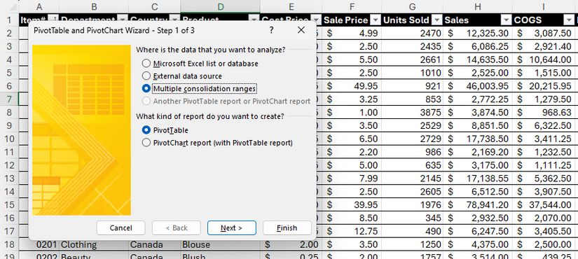
The standard PivotTable wizard isn’t designed to handle multiple, non-contiguous data ranges. This means that the simplest and most accessible path to summary reporting is blocked off as soon as you separate your data onto more than one tab. While the PivotTable Wizard—a legacy tool accessed by pressing Alt > D > P—has the option to combine “Multiple Consolidation Ranges,” this is an outdated feature that still requires tedious, manual range selection across every sheet.

There is an advanced visualization workaround for data stored on multiple worksheets: the Data Model via Power Pivot. However, this is a significant leap in technical difficulty compared to the simplicity of single-data-set PivotTable creation, forcing you to load all sheets and create explicit relationships. There’s also a sense of irony if you spend time learning how to use this tool: it brings all the data into one place, which is precisely what you should have done in the first place to avoid this complex step.

Multi-sheet data filtering becomes a challenge

One of the biggest analytical constraints of having your data fragmented across several tabs is that you can’t easily apply a filter to each worksheet simultaneously.

If you have 12 monthly tabs containing customer details, you can’t run a quick, single filter to find all transactions for a single customer. Instead, you are forced to check 12 individual sheets, applying and clearing the filter each time. While you could solve this with advanced, complex workarounds like writing a VBA macro or using volatile dynamic array functions, the easiest and most robust solution remains the same: consolidate all the data into a single master sheet. This proves that deciding to split the data in the first place is counterproductive.