The BYCOL function acts as a delivery system for a LAMBDA calculation. Here’s how the syntax breaks down:

=BYCOL(array,LAMBDA(c,calculation))

• array is the source data you want to analyze.
• LAMBDA is the engine room where your custom math is built.
• c is the nickname for the current column. As Excel moves through your table, c represents the vertical slice it’s currently looking at. While I’ve used c for clarity, you can actually name this variable anything, as long as you use the same name in your calculation.
• calculation is the math you want to perform on each column.

For example, if A1:D10 contains quarterly sales, this formula returns one average per column:

=BYCOL(A1:D10,LAMBDA(c,AVERAGE(c)))

While BYCOL works with standard ranges (like A1:D50), it thrives on data formatted as an Excel table. However, because dynamic array formulas can’t spill inside an Excel table, place your BYCOL formula outside the table range.

Designing a truly scalable BYCOL formula

Using a formatted Excel table as your source creates a self-expanding system that handles growth automatically. However, to make it truly scalable, you have to be intentional with your references:

• Vertical scalability: As your table grows in length (for example, you add 50 new rows), the BYCOL formula automatically includes that new data. Since the vertical slice (c) simply gets longer, your sums and averages stay accurate without any manual range updates.
• Horizontal scalability: If you reference a specific sub-range like T_Budget[[Q1]:[Q4]], the formula will ignore any new columns added to the right, so point the formula at the entire table using T_Budget[#Data]. However, when you do this, BYCOL will attempt to calculate every column—including the first, which often contains text (like department names or IDs). I’ll show you how to overcome this problem in the scenarios below.

Use case 1: The unbreakable summary row

BYCOL is a powerful safeguard for data integrity. In a standard spreadsheet, anyone can type a manual number over a specific column total, effectively killing the formula for that column. However, because BYCOL houses its logic in a single cell, any attempt to manually type over one of the total cells breaks the spill range and triggers a visible #SPILL! error. This acts as an immediate alert that your summary row has somehow been obstructed, making it harder for someone to hide manual adjustments to your data.

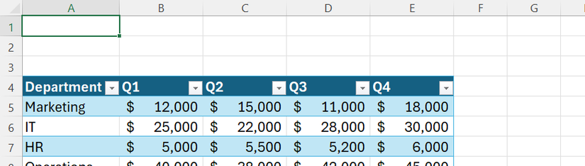
Scenario: You’re managing a departmental budget tracker (named T_Budget) and need a horizontal total row that stays pinned to the top of your sheet.

Here’s the formula you’ll need to type in cell A1:

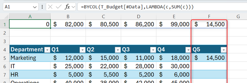
=BYCOL(T_Budget[#Data],LAMBDA(c,SUM(c)))

This formula tells Excel to look at every column in the T_Budget table. It defines each column as c, and the LAMBDA instructs Excel to sum the values. Because you used [#Data], if you add a Q5 column, the formula will automatically detect it and spill one cell further to the right.

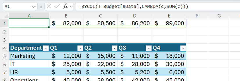
However, because the Department column contains text, the first result of your BYCOL formula is 0. To hide this zero without breaking the formula’s scalability, select the cell containing the zero, press Ctrl+1 to open the Format Cells dialog, select Custom, and type ;;; (three semicolons) in the Type box.

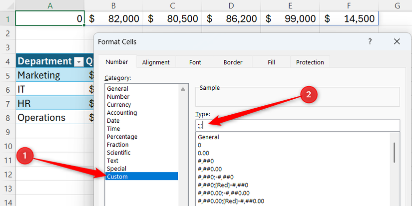
When you click “OK,” the value disappears.

The benefits of BYCOL in this scenario

• vs. legacy functions: A standard SUM dragged across multiple cells is vulnerable. If someone manually overwrites a total to “fix” a budget gap, the error remains hidden. However, with BYCOL, if any part of the spilled range is tampered with, the whole row triggers a #SPILL! alert.
• vs. the table total row: Excel tables let you add a total row to the bottom (Table Design > Total Row). However, in a large table with thousands of rows, they’re invisible unless you scroll down. BYCOL allows you to park your totals at the top of the sheet so they stay frozen in view as the table grows.

Use case 2: Vertical logic checks (checkboxes)

While Excel tables offer a wide range of built-in summary tools—ranging from averages and counts to standard deviations—they’re primarily designed to aggregate data at the foot of a table. They don’t have a native, spill-friendly way to evaluate complex conditions down an entire column and report a dynamic status elsewhere, like in a dashboard header at the top of your sheet. But BYCOL can.

Scenario: You’re managing a multi-stage project launch where several team members are assigned tasks in each phase. You want a status indicator above your T_Projects table that only marks a phase as “Complete” when every person in that column has checked their box.

To keep your indicators scalable for when you inevitably add a Phase 4 column—and to prevent errors in cell A1—use this formula:

=BYCOL(
T_Projects[#Data],
LAMBDA(c,
IF(ISERROR(AND(c)),"",
IF(AND(c),"Complete","In Progress"))
))

Here’s how this formula works:

• ISERROR(AND(c)),””: Unlike SUM, logical functions like AND can’t ignore text. If the formula tries to process the Team Member column, it fails. This logic gate tells Excel that if an error occurs (because of text), it should return an empty string (“”) instead of a #VALUE! error.
• IF(AND(c)…): For columns containing logical values (the checkboxes), the formula proceeds as normal. The AND function checks if every single team member’s box is checked and, if so, returns “Complete.” If just one box is unchecked, it shows “In Progress”.