
Situatie
Excel usually warns you about obvious formula mistakes, but some of the most damaging errors never trigger an alert. From shifting cell references to hidden lookup failures, these silent bugs can skew your results while leaving your spreadsheet looking perfectly normal.
Solutie
Switch to absolute references for fixed variables
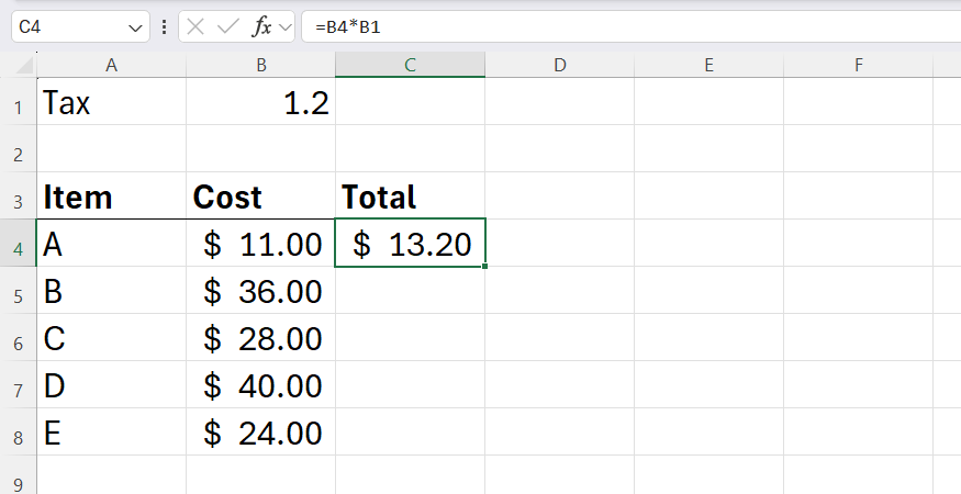
When you build a formula and use the fill handle to copy it down a column, Excel automatically increments the row numbers in your cell references. This is helpful when you’re calculating line-by-item totals, but it breaks your calculations if your formula needs to reference a single fixed variable like a tax rate, discount percentage, or shipping fee.
For example, copying the formula:
=B4*B1
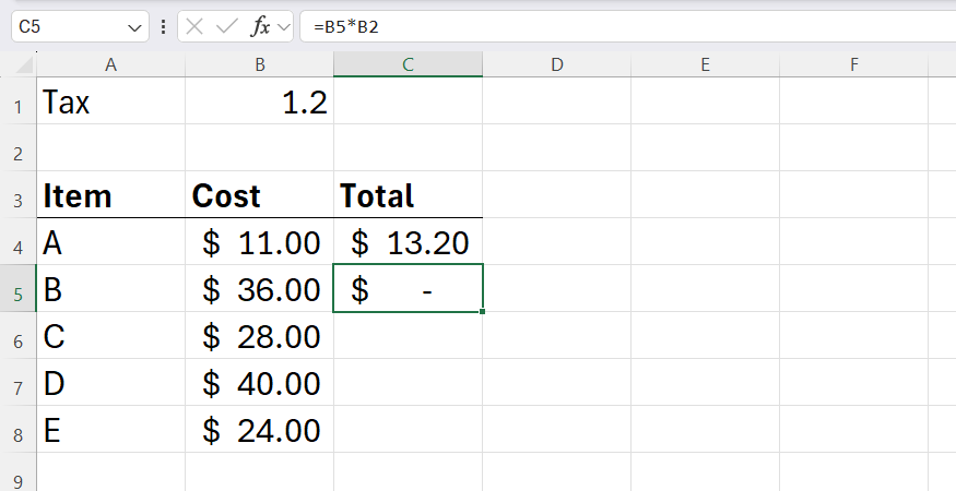
down one row changes it to:
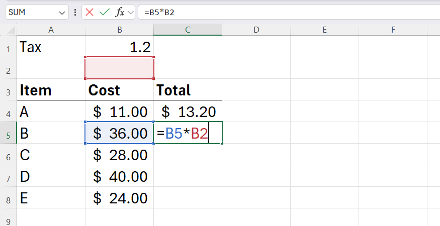
=B5*B2
If cell B2 is empty, Excel treats it as a zero, so your formula returns an incorrect calculation instead of throwing an explicit error.
To fix this, anchor the cell reference:
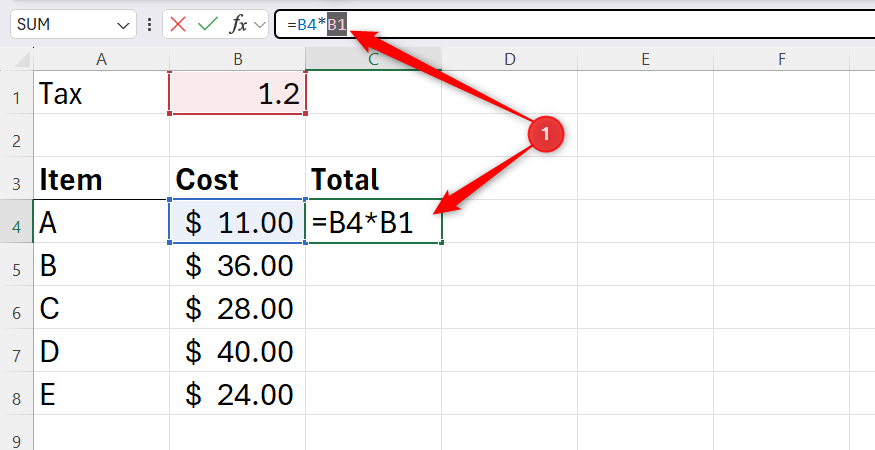
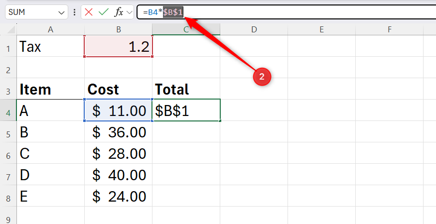
- In the formula bar, select the specific cell reference that needs to stay frozen.
- Press F4 once to insert dollar signs around the coordinates.
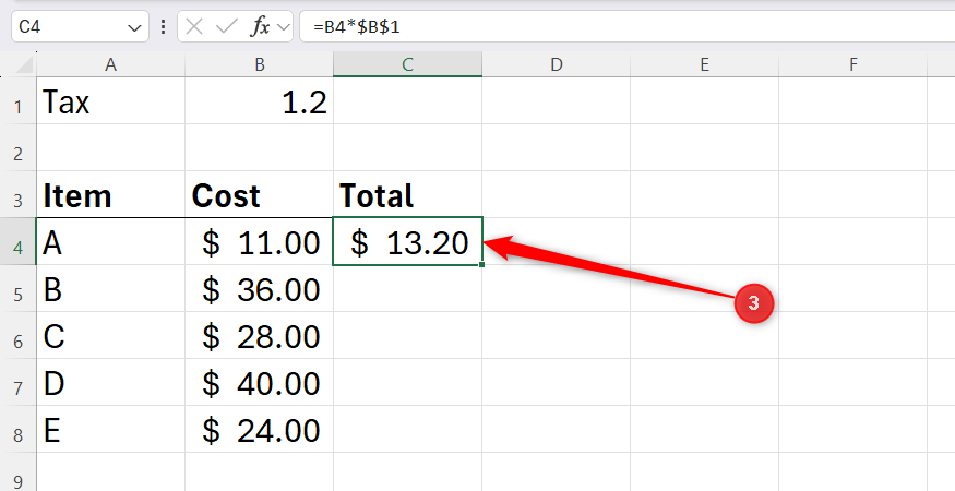
- Press Ctrl+Enter to commit the formula and keep that cell selected.
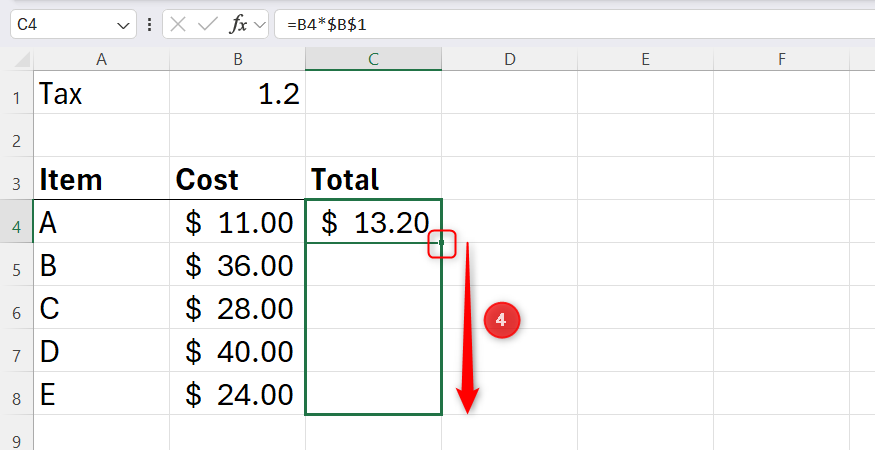
- Drag the fill handle down to apply the locked formula to the rest of your column.
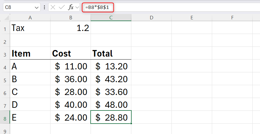
Once updated, your formula will continue referencing the correct value throughout the column:
=B8*$B$1
Clean up your data with a simple function
Leading and trailing spaces don’t affect standard mathematical functions like SUM or AVERAGE because Excel generally ignores them during numeric calculations. But text-based operations, logical tests, and lookups evaluate your data entirely literally.
If you write a logical test like:
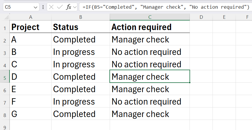
=IF(B2="Completed", "Manager check", "No action required")
and drag it down a column, but a target cell contains ” Completed” (with a leading space), Excel returns the wrong result without triggering an alert or error flag.
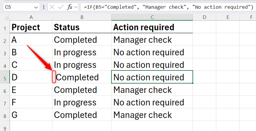
To remove hidden leading or trailing spaces from your text strings, use the TRIM function:
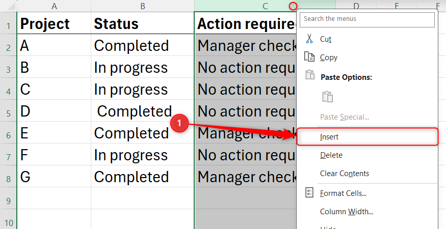
- Insert a temporary blank column directly next to your text entries.
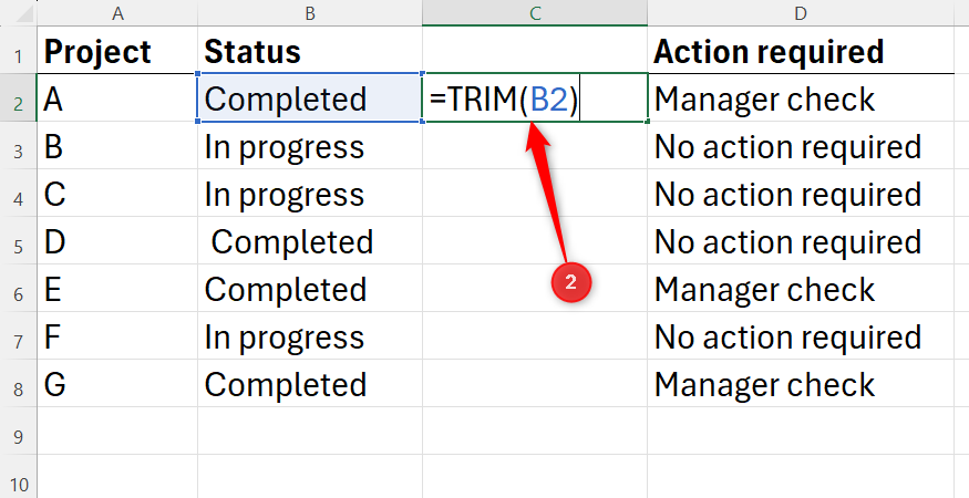
- Type:
=TRIM(B2)
into the first empty cell, replacing “B2” with your first target cell reference.
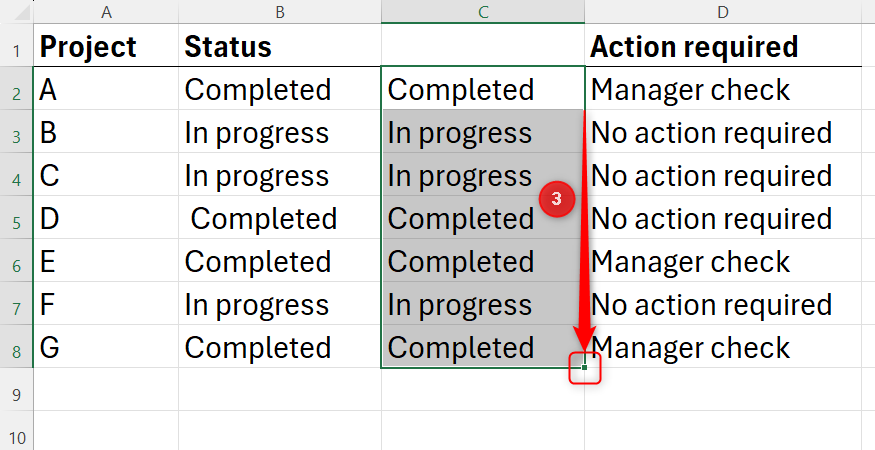
- Press Ctrl+Enter and drag the formula down to the bottom of your data block.
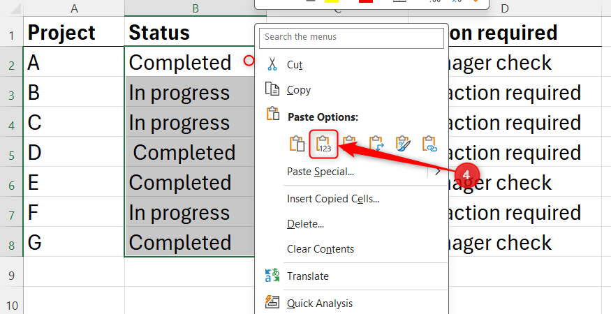
- Copy the new values, select and right-click the original data column, and click Paste as Values (or press Ctrl+Shift+V).
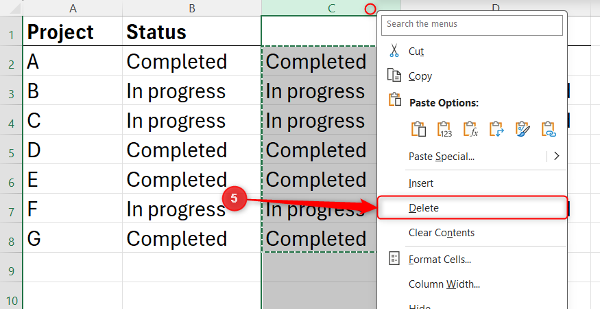
- Delete the temporary column.
Now that those ghost spaces are trimmed, your logic works as expected.
Hard-coded column indexes break when layouts shift
Give your workflow a facelift with modern functions
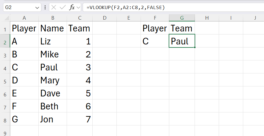
Legacy lookup functions require you to hard-code a static index number to tell Excel which column to pull data from, making your formulas highly vulnerable to structural changes.
If you write a formula like:
=VLOOKUP(E2,A2:B8,2,FALSE)
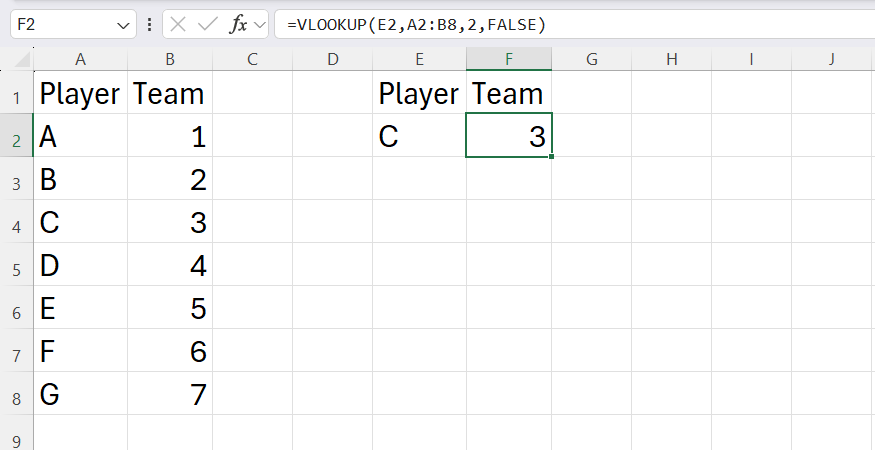
You can fix this by upgrading your spreadsheet to XLOOKUP, which targets specific source and return ranges instead of counting columns:
- Select your target cell and type:
=XLOOKUP(
- Select the cell containing the value you want to search for, then type a comma.
- Select the range containing that search key, then type a comma.
- Select the range containing the data you want to return.
- Close the parentheses, and press Ctrl+Enter.
Your completed formula will look like this:
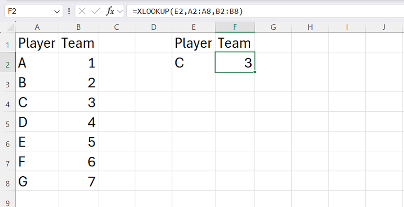
=XLOOKUP(F2,A2:A8,C2:C8)


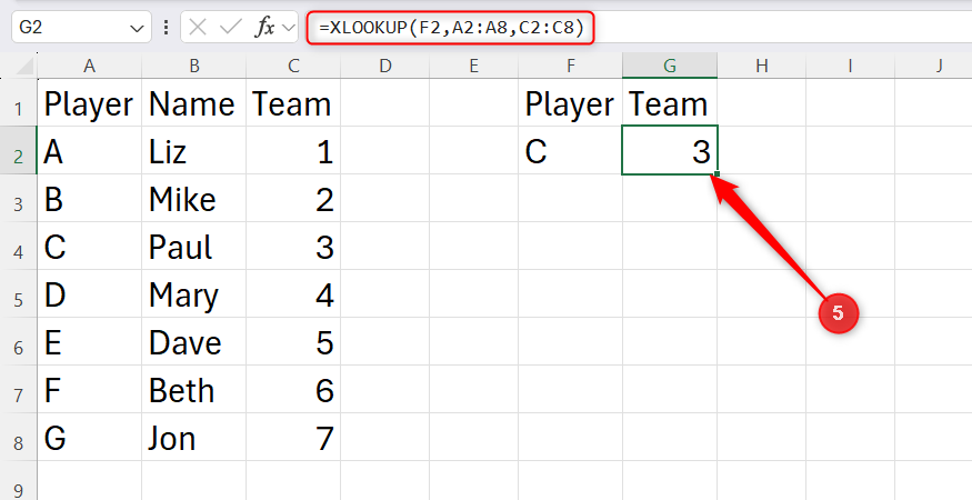
Because it uses separate lookup and return ranges instead of a fixed column index, it avoids VLOOKUP’s structural fragility and continues returning the correct field as the sheet changes.
Use targeted error handling instead of IFERROR
Wrapping formulas inside an IFERROR statement is a quick way to clean up your worksheet when it starts filling with error codes. The problem is that IFERROR treats every error the same way—it doesn’t distinguish between expected lookup failures and structural spreadsheet errors.
This becomes dangerous when IFERROR hides problems you actually need to see. For example, a formula like:
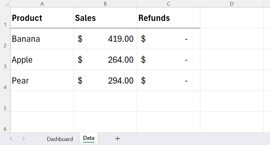
=IFERROR(SUM(INDEX(Data!B2:C4,,MATCH(Dashboard!C3,Data!B1:C1,0))),0)
appears harmless, but if the Data worksheet is deleted, the formula will silently return 0 instead of exposing a #REF! error.
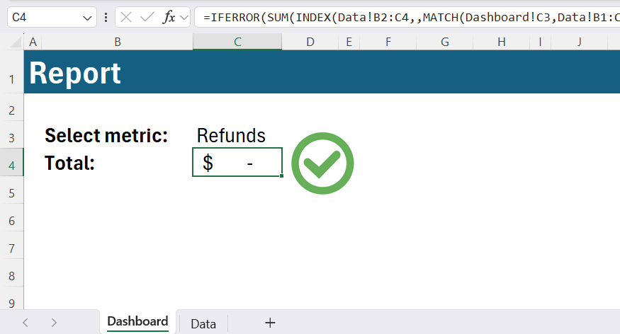
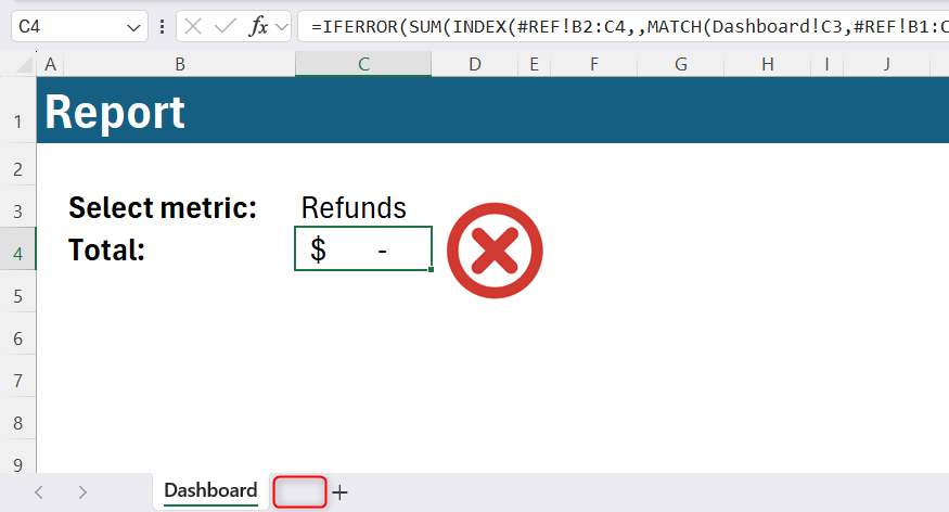
Rather than wrapping every formula in IFERROR, use it only when all errors should genuinely produce the same result. Otherwise, leave the error messages visible so you can identify and fix real calculation problems before they affect your reports.
If you’re only handling missing lookup results, use a more targeted approach like IFNA to catch #N/A errors, or modern functions like XLOOKUP, which include a built-in “if not found” argument that lets you define fallback behavior without hiding unrelated calculation errors.
Standard summary functions ignore what’s visible
SUBTOTAL to the rescue
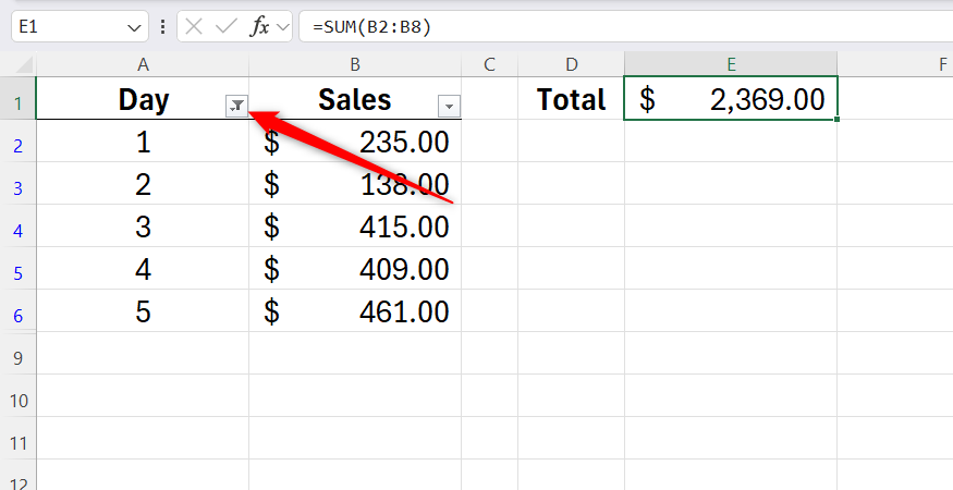
When you’re working with manually hidden or filtered-out rows, standard summary functions like SUM and AVERAGE still calculate the entire range, even when those rows aren’t visible. This creates a mismatch between what you see on screen and what Excel is actually totaling.
For example, if you type:
=SUM(B2:B8)
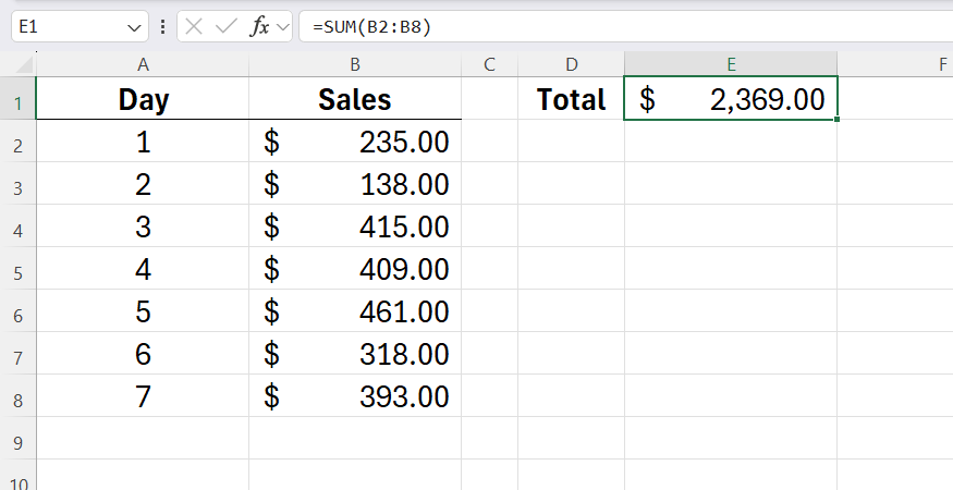
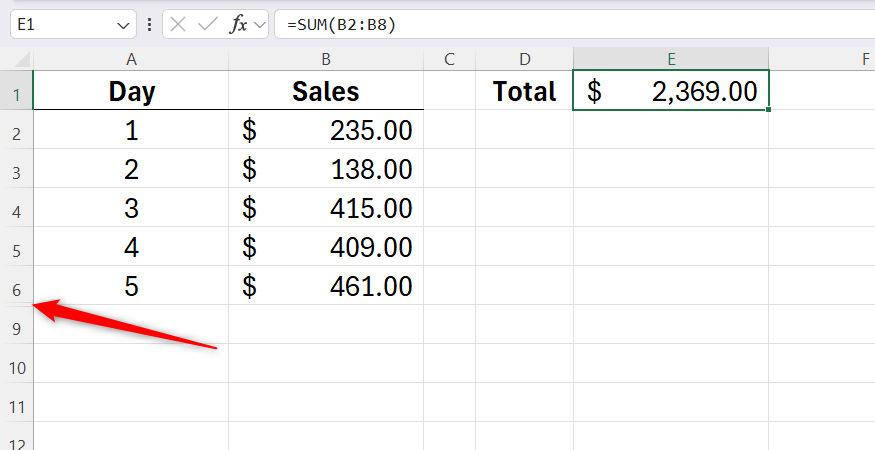
To ensure your totals reflect only visible data, switch to the SUBTOTAL function:
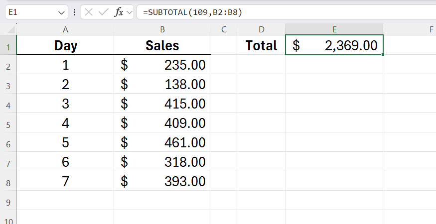
=SUBTOTAL(109,B2:B8)
replacing “109” with the operation you need per the table below. Using 109 for SUM ensures your totals exclude both filtered-out rows and manually hidden rows, keeping your results aligned with what is currently visible.
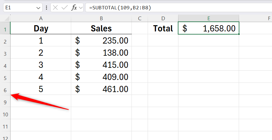
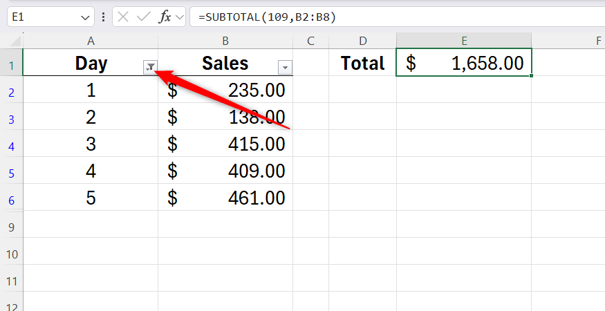
The function number controls how Excel treats manually hidden rows:
Leave A Comment?