How to use the REGEX functions in Excel

Situatie

Regular expressions (or REGEX) are search patterns that can be used to check if a string of text conforms to a given pattern and extract or replace strings of text that match a given pattern. Given their complexity, this article offers streamlined summaries and examples of their use in Excel.

Solutie

Pasi de urmat

This function tests whether a string of text matches a given pattern, returning TRUE or FALSE based on this test. This is a great way to test that your data follows a certain pattern.

REGEXTEST(a,b,c)

where

a (required) is the text, value, or cell reference containing the text you want to test,
b (required) is the pattern used to perform the test, and
c (optional) is either 0 if you want the test to be case-sensitive, or 1 if not.

Example of How to Use REGEXTEST

This spreadsheet contains a list of product codes that must follow a strict structure.

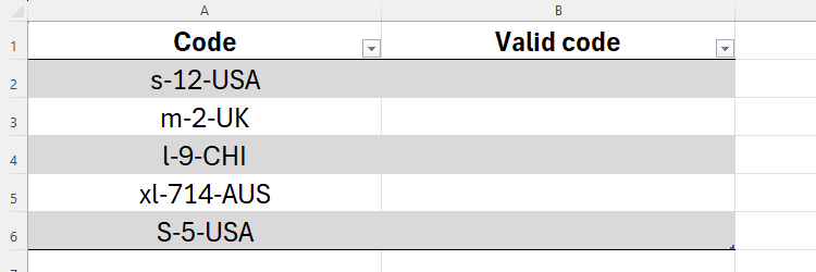
A valid code contains:

A lowercase representation of the product size (“xs” for extra-small, “s” for small, “m” for medium, and so on),
A one or two-digit number representing the product’s material,
Three uppercase letters that represent where the product is manufactured, and
A dash between each of the three parts described above.

I want to test that all the product codes match this structure.

So, in cell B2, I will type:

=REGEXTEST([@Code],"[xs|s|m|l|xl]-[0-9]{1,2}-[A-Z]{3}",0)

where

[@Code] is a structured reference to the column where the codes I want to test are located,
[xs|s|m|l|xl] is the first part of the product code I want to test, with the vertical lines meaning “or”,
[0-9]{1,2} is the second part of the product code I want to test, with [0-9] being any single digit, and {1,2} meaning there can be one or two single digits,
[A-Z]{3} is the third part of the product code I want to test, with [A-Z] being any uppercase letter, and {3} meaning there need to be exactly three of these,
The three parts of the code I want to test are separated by a dash, and
0 is the final argument in the formula that tells Excel the test is case-sensitive.

When I press Enter to apply this formula to all rows in column B, the result reveals that only two of the codes are valid (TRUE).

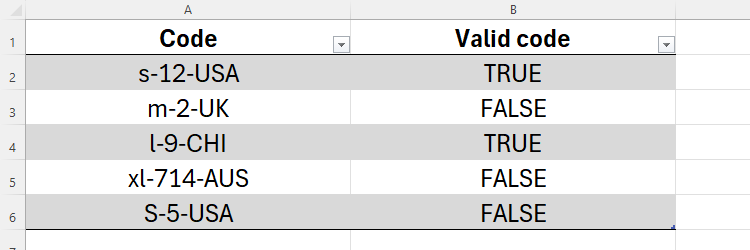
A list of product codes in Excel, and a second column that tests whether the code is valid using the REGEXTEST function.

m-2-UK is invalid (indicated by the FALSE result) because the country code only contains two uppercase letters
xl-714-AUS is invalid because the material code contains three digits, and
S-5-USA is invalid because the size code is uppercase.

This example contains the use of characters like [ ] and { }. However, there are many more characters (also known as tokens) that can also be used to determine the pattern used to perform the test, some of which I’ll use in the examples below.

This function returns parts of text in a cell according to a specified pattern. For example, you might want to separate numbers and text.

Syntax

REGEXEXTRACT(d,e,f,g)

where

d (required) is the text, value, or cell reference containing the text you want to extract from,
e (required) is the pattern you want to extract,
f (optional) is 0 if you want to extract the first match only, 1 to extract all applicable matches as an array, and 2 to extract groups from the first match, and
g (optional) is either 0 if you want the extraction to be case-sensitive, or 1 if not.

Because formatted Excel tables can’t handle spilled arrays, if you intend to extract matches as an array in argument f, make sure your data is plainly formatted.

Example of How to Use REGEXTRACT

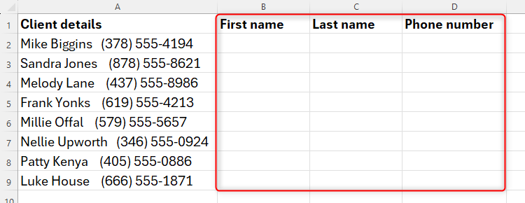
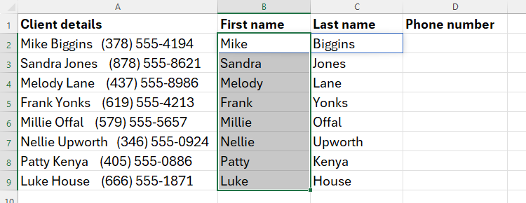
In this example, I want to extract the clients’ first names, last names, and phone numbers into three separate columns.

An Excel spreadsheet containing a list of names and phone numbers in column A, and subsequent columns created where the information will be extracted through REGEXEXTRACT.

Let’s focus on the names first. In cell B2, I will type:

=REGEXEXTRACT(A2,"[A-Z][a-z]+",1)

where

A2 is the cell containing the data I want to extract,
[A-Z][a-z]+ tells Excel that I want to extract any words that start with a capital letter followed by lowercase letters, with the “+” indicating that I want to return one or more lowercase letters in each pattern, and
1 indicates that I want each example of the above pattern to be separated into individual cells as an array (in other words, the first name in cell B2, and the second name in cell C2). If I omitted this argument, Excel would return the first match (the first name) only in cell B2.

When I press Enter, Excel performs the extraction successfully and adds a faint blue line around cell C2 to remind me that it’s a spilled array.

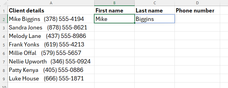
An Excel spreadsheet containing a first name and surname extracted into cells B2 and C2 from cell A2 using REGEXEXTRACT.

With cell B2 selected, I can now use the fill handle in the bottom-right corner of the cell to duplicate this relative formula to the remaining rows of details.

A series of first and last names have been extracted in Excel from column A to columns B and C using REGEXEXTRACT.

Now, I need to use a similar REGEXTRACT formula to extract the clients’ phone numbers. In cell D2, I will type:

=REGEXEXTRACT(A2,"[0-9()]+ [0-9-]+")

where

A2 is the cell containing the data I want to extract,
[0-9()]+ extracts digits from zero to nine that are inside rounded parentheses, with the “+” extracting one or more digits in this pattern, and
[0-9-]+ extracts the remaining digits from the string, with the second “-” representing the dash that separates the two parts of the phone number, and the “+” telling Excel that I want to extract one or more digits if the string contains them.

Since there is only one instance of this pattern in each cell in column A, I don’t need to add any more arguments. Again, once I’ve checked that this formula produces the expected result, I can use the fill handle to duplicate it to the remaining cells in column D.

There are other ways in Excel to extract data and achieve similar results, such as using the TEXTSPLIT function or Excel’s Flash Fill tool.

This function takes text in a cell and creates a new version of that data in another cell. Even though the function is called REGEXREPLACE, it doesn’t actually replace the original text in its original location.

Syntax

REGEXREPLACE(h,i,j,k,l)

where

h (required) is the text, value, or cell reference containing the text you want to replace,
i (required) is the pattern you want to replace,
j (required) is the replacement you want to create,
k (optional) is the occurrence of the pattern you want to replace, and
l (optional) is either 0 if you want the replacement to be case-sensitive, or 1 if not.

Example of How to Use REGEXREPLACE

Below, you can see a list of names in column A. My aim is to recreate these names in column B, but using the “Last name, First name” format, including the comma separating the names.

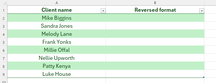
A list of names in column A in Excel, with the empty column B headed 'Reversed format'.

In cell B2, I will type:

=REGEXREPLACE([@Client name],"([A-Z][a-z]+) ([A-Z][a-z]+)","$2, $1")

where

[@Client name] references the column containing the data I want to affect,
[A-Z][a-z]+ being included twice in the formula (and separated by a space) tells Excel that I want to take the two strings of text that contain a capital letter followed by one or more lowercase letters, and
$2, $1 tells Excel that I want to reverse the order of those two strings of text, separated by a comma and a space. If I didn’t include the dollar symbols, Excel would simply return “2, 1” as the result in each cell.

Tip solutie

Permanent

Follow Us