I upgraded my Excel PivotTable with these 3 simple features

Situatie

I’m probably guilty of making Excel spreadsheets more complicated than they need to be, but I have one rule I keep coming back to: if I’m going to build a PivotTable, I want to actually enjoy using it. The basic summary is useful, but a few small additions can make a surprisingly big difference.

After converting my data into a table with Ctrl+T, creating a PivotTable in a new worksheet via Insert > PivotTable, and dragging fields into the different areas of the PivotTable Fields pane, it’s easy to stop there. But that’s only the start. I usually add three simple features—slicers, timelines, and PivotCharts—to make the results easier to filter, explore, and understand.

For the examples in this article, I’m using a fictional 500-row sales ledger. You can download a free copy of this worksheet to try the three features yourself. When you click the link, you’ll find the download button in the top-right corner.

Solutie

Slicers make my PivotTables much easier to control

I like being able to see my filters

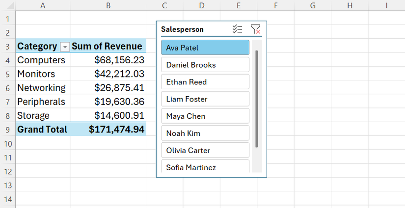
In Microsoft Excel, a PivotTable updates revenue values after selecting Ava Patel in the Salesperson Slicer.

The first thing I tend to add to a PivotTable is a slicer. I like being able to see exactly how I’ve filtered my data, rather than opening a small drop-down menu and trying to remember which options I’ve selected. I also like that I can use a slicer to filter by a field that isn’t actually visible in the PivotTable, giving me another way to explore the same summary.

For my sales ledger, I started with a PivotTable showing Revenue by Category. I clicked inside the PivotTable, went to PivotTable Analyze > Insert Slicer, and selected Salesperson. Excel added a set of buttons for the eight salespeople in my dataset, and clicking Ava Patel, for example, immediately filtered the PivotTable to show only her sales.

In Microsoft Excel, a PivotTable shows Category and Sum of Revenue with the Computers row highlighted.

In Microsoft Excel, the PivotTable Analyze tab is highlighted on the ribbon.

In Microsoft Excel, the Insert Slicers dialog box appears over a PivotTable, with the Salesperson checkbox selected.

In Microsoft Excel, a Salesperson Slicer is displayed next to a PivotTable, with Ava Patel highlighted.

In Microsoft Excel, a PivotTable updates revenue values after selecting Ava Patel in the Salesperson Slicer.

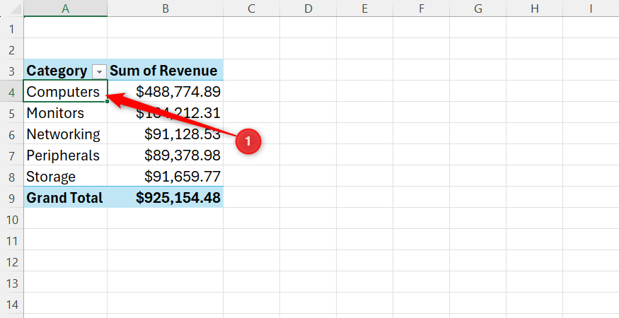
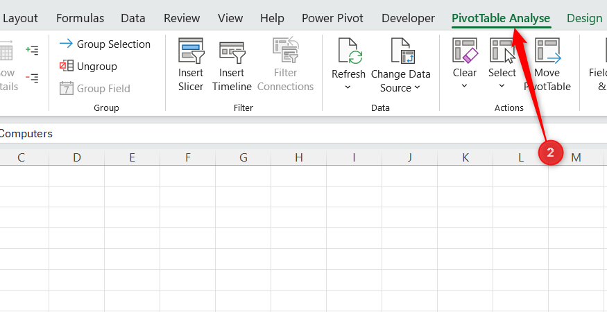
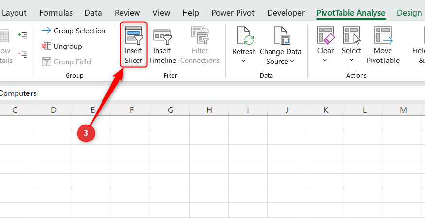
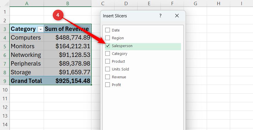
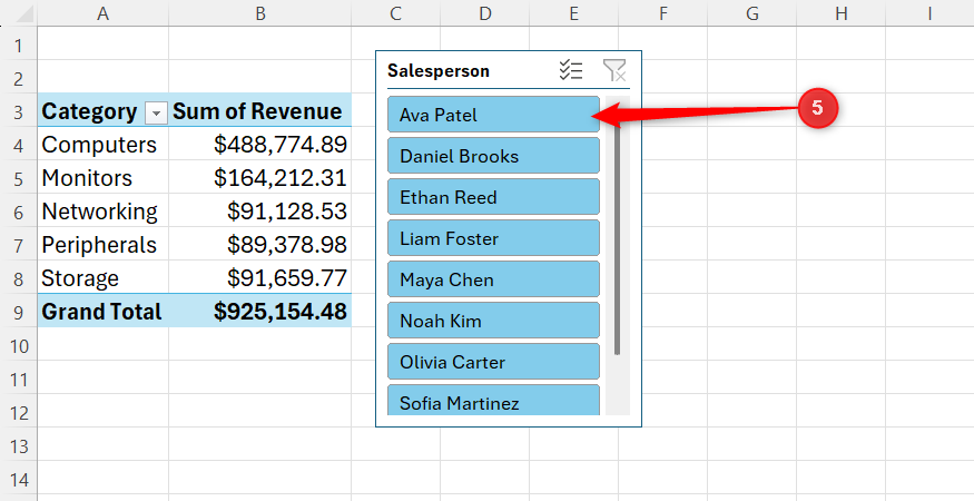
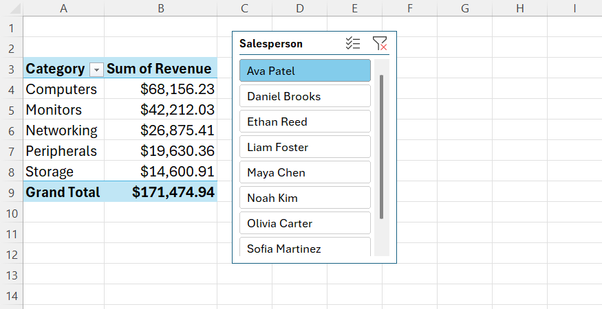
I can select multiple salespeople by holding Ctrl while clicking, or clear my selection using the Clear Filter button in the top-right corner of the slicer.

Slicers aren’t exclusive to PivotTables—you can add them to a regular Excel table—but I find them particularly useful with PivotTables because one slicer can control multiple PivotTables based on the same source data.

In my case, I created a second PivotTable showing Revenue by Region. I then right-clicked my Salesperson slicer, selected Report Connections, checked the box for my Region PivotTable, and clicked OK. Now, whenever I click a salesperson, both PivotTables update at the same time.

In Microsoft Excel, a second PivotTable showing revenue by region is highlighted next to the original PivotTable and Slicer.

In Microsoft Excel, the Report Connections dialog box has both PivotTable options selected to connect to the Slicer.

In Microsoft Excel, selecting Ava Patel in the Slicer updates revenue data across both connected PivotTables.

In Microsoft Excel, selecting multiple names in the Slicer updates revenue data across both connected PivotTables.

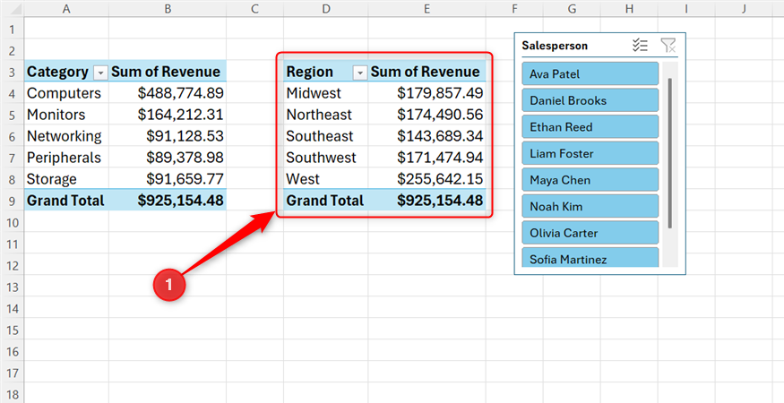
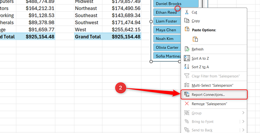
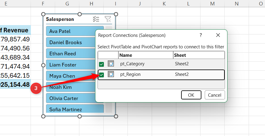
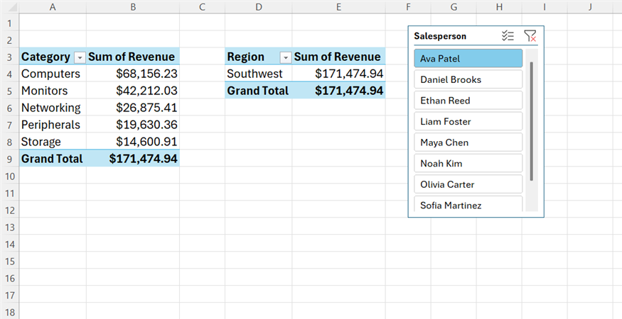
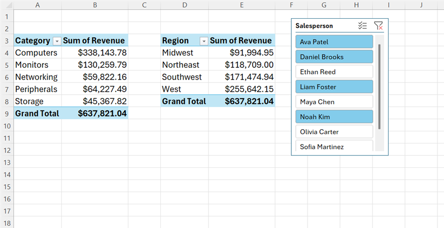
That’s the part I really like. Instead of opening separate filter menus for each PivotTable, I have one set of visible buttons that lets me control the summaries I’m looking at.

A timeline makes date filtering much less fiddly

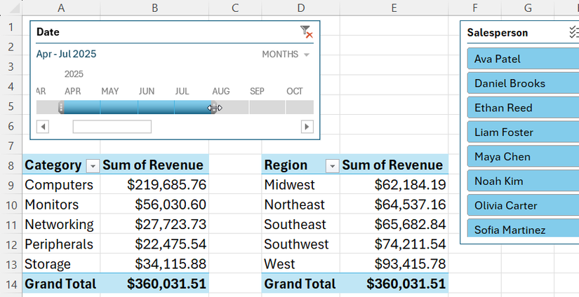
In Microsoft Excel, the cursor drag selects the timeline filter to cover Apr to Jul 2025 above two connected PivotTables.

Dates are one of the first things I often want to filter when I’m looking at my data, but the standard PivotTable date filter isn’t my favorite way to do it. When I have a whole year’s worth of records, scrolling through individual dates feels cumbersome.

Your source data must contain actual Excel dates for a timeline to work. Dates that look like dates but are stored as text won’t be recognized correctly.

That’s why I usually add a timeline. I went back to my first PivotTable and clicked PivotTable Analyze > Insert Timeline. I then selected Date, clicked OK, and Excel added a timeline showing the 2025 sales data. Because I had two linked PivotTables, I also right-clicked the timeline, selected Report Connections, and checked the box for my Revenue-by-Region PivotTable.

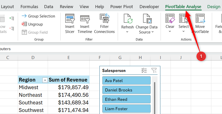
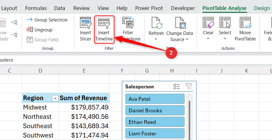
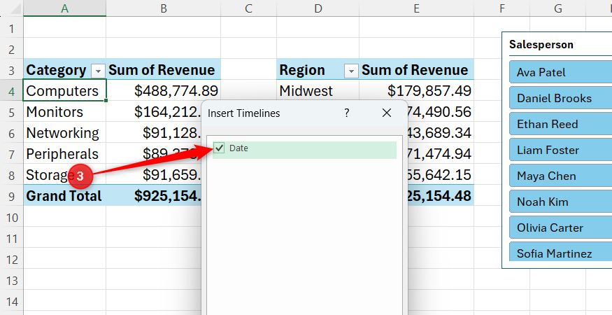
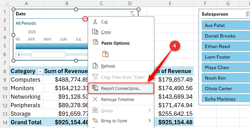
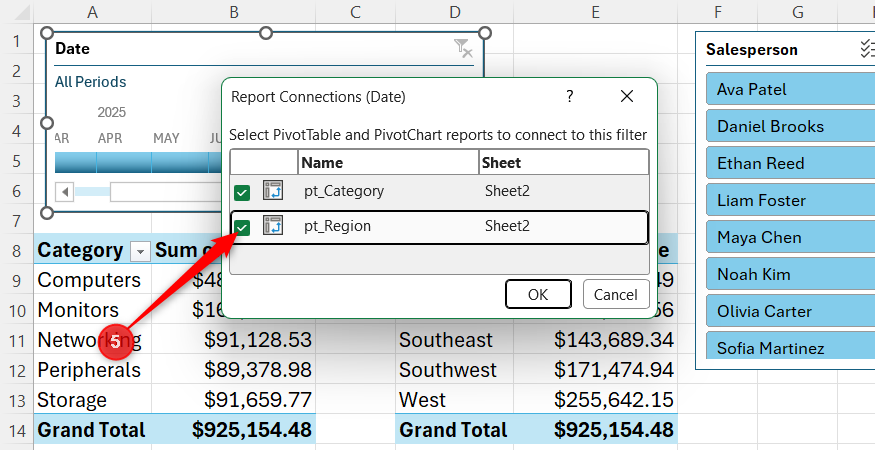
In Microsoft Excel, the Insert Timelines dialog box appears over two PivotTables, with the Date checkbox selected.

In Microsoft Excel, the Report Connections dialog box has both PivotTable options selected to connect to a timeline.

Timelines let you filter the PivotTable by Years, Quarters, Months, or Days. I usually stick with Months for a dataset like this. Then, instead of opening a filter menu and selecting individual dates, I can simply click a month or drag across several months to create a date range. For example, I can drag from April through July and immediately see how my PivotTables change to reflect those four months.

The timeline also works alongside my slicer. If I select Ava Patel in the Salesperson slicer and then drag across a few months in the timeline, I can quickly narrow both connected PivotTables down to Ava’s sales during that particular period.

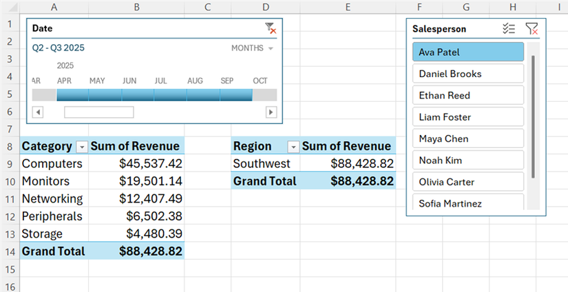
In Microsoft Excel, a Slicer and timeline filter two PivotTables to show Ava Patel's sales for April to Sep 2025.

I find that much easier to work with than repeatedly opening filter menus. The timeline also makes it obvious which period I’m looking at, which is particularly useful when I come back to the spreadsheet later.

PivotCharts show me what my numbers are actually doing

Sometimes a table of numbers needs a picture

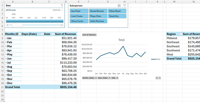
In Microsoft Excel, a line PivotChart sits between two PivotTables, below a timeline and a Salesperson Slicer.

I like being able to see the actual figures in my PivotTable, but sometimes I want to spot a trend without having to study a column of numbers. That’s when I add a PivotChart.

For this example, I wanted to see how my sales changed throughout 2025, so I went back to my Revenue-by-Category PivotTable, clicked PivotTable Analyze > PivotChart, and chose a Line chart. I then removed Category from the Rows area and used Date instead, while keeping Revenue in the Values area. This gave me a single line showing total sales for each month of 2025.

In Microsoft Excel, the Computers cell in a PivotTable is highlighted beneath a timeline and a Slicer.

In Microsoft Excel, the Line option is selected in the Insert Chart dialog box over a PivotTable.

In Microsoft Excel, the Remove Field option is highlighted for the Category row in the PivotTable Fields pane.

In Microsoft Excel, checking Date in PivotTable Fields adds Months, Days, and Date drop-down fields under Rows.

In Microsoft Excel, a line PivotChart sits between two PivotTables, below a timeline and a Salesperson Slicer.

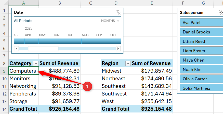
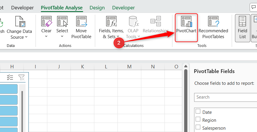
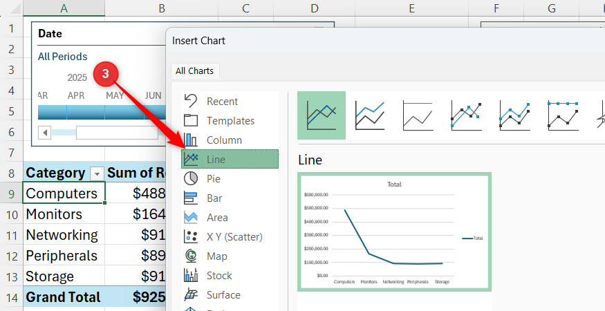
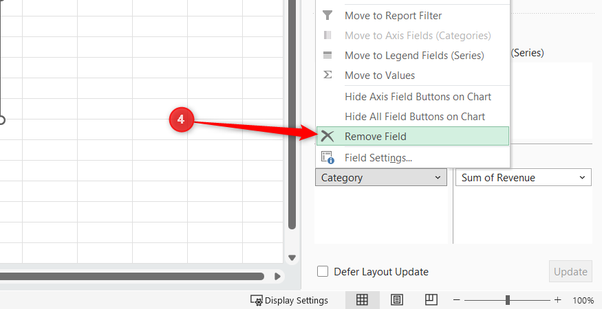
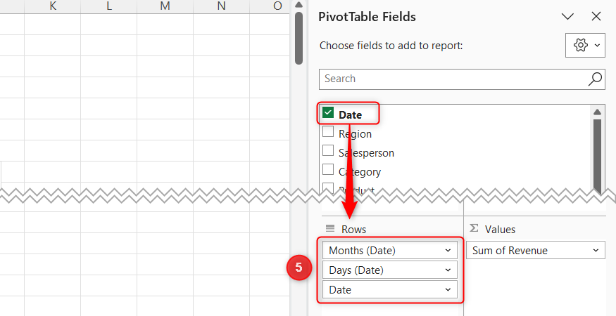
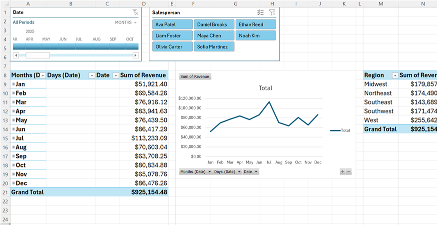
Keep an eye on the Rows area of the PivotTable Fields pane when adding a Date field. Excel can add things like Days (Date) to your PivotTable. If you don’t want them included, drag them out of the Rows area.

The useful thing about a PivotChart is that it stays connected to the PivotTable. I can use the field buttons around the chart to change what I’m viewing, and those changes are reflected in the PivotTable too.

My Salesperson slicer and timeline are connected as well. If I select Ava Patel in the slicer, the chart immediately changes to show only her sales. I can also use the timeline to narrow it down to a few months.

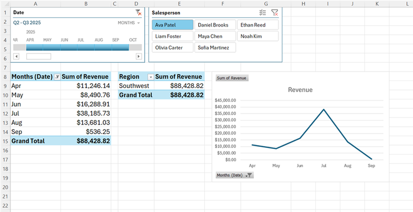
In Microsoft Excel, selecting Ava Patel for Q2 to Q3 2025 updates two PivotTables and a line PivotChart.

That means I don’t have to create a separate chart every time I want to look at a different slice of the data. I can use the chart controls, slicer, or timeline to change what I’m looking at, while the PivotChart gives me an immediate visual representation of the result.

A few small additions can make a big difference

A basic PivotTable is only the starting point. Slicers make filtering easier, timelines make date ranges easier to explore, and PivotCharts help me spot trends at a glance. Once everything is set up, I can use PivotTable conditional formatting to highlight the numbers that matter. I also make use of a few little-known PivotTable tricks to take them to the next level, like generating separate worksheets for each category, using distinct counts to track unique values, and calculating month-over-month growth without using any formulas.

Tip solutie

Permanent

Follow Us