Using the Text to Columns Tool

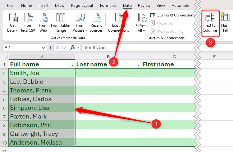
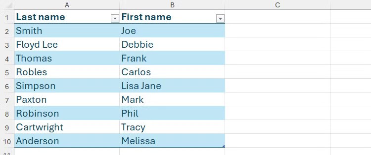
One way to split data into multiple columns in Microsoft Excel is to use the built-in Text To Columns tool. This method is handy if you prefer to work in a dialog box that guides you through the process. For example, let’s say you want to split the names in column A into last and first names in columns B and C, respectively.

To do this, first, select the cells in column A, and in the Data tab on the ribbon, click “Text To Columns”

In the Convert Text to Columns Wizard, select “Delimited,” and click “Next”

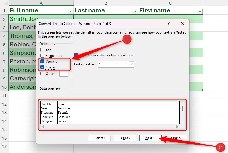
A delimiter is a character, symbol, or space that is used to separate items in a sequence. In this example, the names in column A are separated by a comma and a space, so check both these options. You can see how this will affect your data in the preview at the bottom of the dialog box. If you’re happy, click “Next”.

Next, clear any information in the Destination field, select the cell where you want the split data to be—in this case, cell B2—and click “Finish”.

Now, the full names are split into last and first names in their respective columns. If needed, you can delete the original data in column A, as the split names aren’t linked in any way to the full names.

However, in this example, one person has two first names, and another person has two surnames. In this case, selecting the space delimiter will split these dual names into separate columns, even though you want to keep them together.

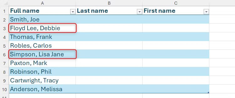
To overcome this, select the comma delimiter only—not the space delimiter—in the Convert Text to Columns Wizard.

Once the splitting process is complete, however, you’ll notice that the first names are preceded by a space, as you didn’t tell Excel to consider spaces as delimiters.

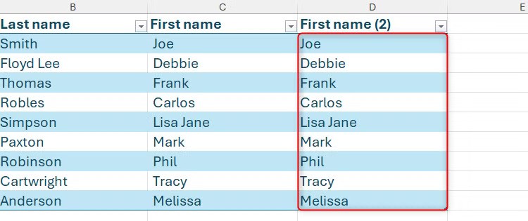
To remove these spaces, expand the table one column to the right to create another column for the corrected first names. Then, in cell D2, type:  =TRIM([@[First name]])

where the TRIM function removes all spaces from a text string (except for spaces between words), and [@[First name]] is a structured reference to the column in the table called “First names.”

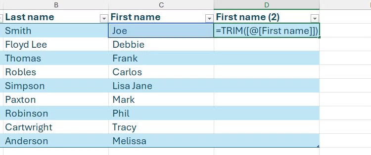
When you press Enter, the first names will appear in column D, but this time, without the leading space. Also, because the data is in a formatted Excel table, the formula is duplicated automatically in the remaining cells of the column.

Next, select the newly generated first names, and press Ctrl+C to copy them. Now, press Ctrl+Alt+V to open the Paste Special dialog box, then V to select “Values,” then Enter.

Finally, delete the column containing the spaces before the first names (C) and the original column containing the full names (A) to complete your table.