You might be familiar with bookmarks in Microsoft Word, which are invisible way-points in specified locations of a document that you can jump to whenever you need to. Microsoft Excel’s alternative to this time-saving tool is somewhat unimaginatively called “names,” accessed through the name box in the top-left corner of your workbook.

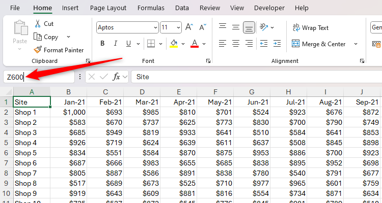
Let’s say you have a huge worksheet containing lots of rows and columns of data, and you want to jump to a certain cell without scrolling for what seems like forever. The quickest way to do this is to type a cell reference in the name box and press Enter.

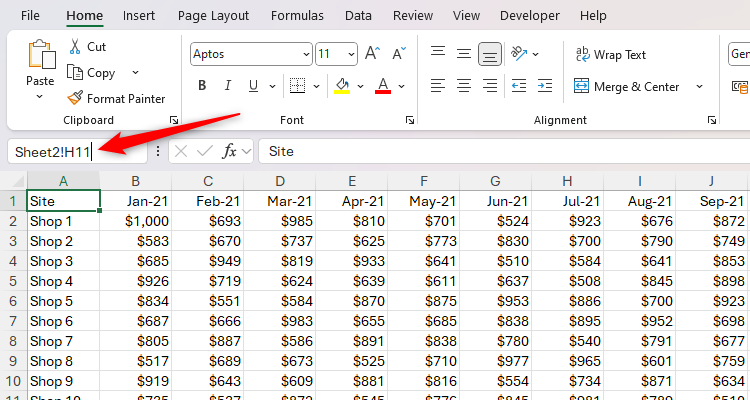
Likewise, if you have other active tabs in your workbook, you can jump to any cell within any of the worksheets by typing the tab name, followed by an exclamation mark, and then cell reference. For example, typing:

Sheet2!H11

and pressing Enter takes you to cell H11 in Sheet 2.

While this is all well and good, it’s of little use if you can’t remember which cells contain the information you want to jump to. This is why you should change the names of cells or ranges that you will either visit or use in formulas often.

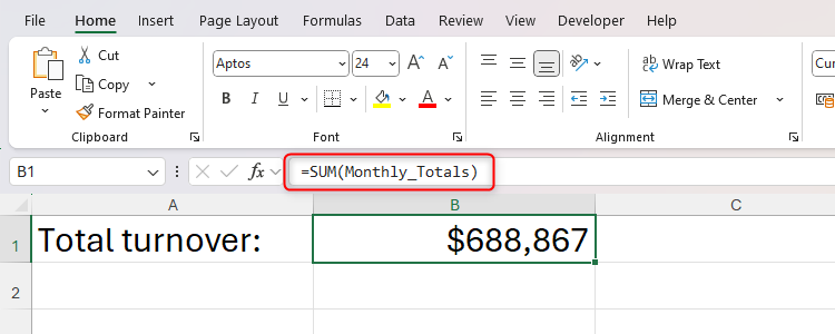
In this example, I have named a range of cells “Monthly_Totals” that I review all the time. Because I’ve named the range, I can jump to it by clicking the down arrow in the name box, regardless of which worksheet I’m currently working in.

What’s more, I can use this named range in a formula. For example, typing:

=SUM(Monthly_Totals)

adds all the values in this range and provides an overall total.

As a result of using a named range rather than direct cell references, I can guarantee that I’ve not accidentally selected the wrong cells. What’s more, because the referenced range has a descriptive name, when I look at the formula, it’s easy to remind myself of how the calculation is made. A third benefit of using named ranges in formulas is that they’re easier to troubleshoot if the figure doesn’t seem quite right.

Another good example of the usefulness of named ranges in formulas is when they form part of a logical test in the IF function. In this example, by clicking the cell and looking in the formula bar, you can immediately see that the criterion for whether the threshold is met involves the total income. On the other hand, using cell references here would make this less clear:

=IF(Total_Income>10000,"Threshold met","Threshold not met")

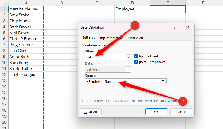
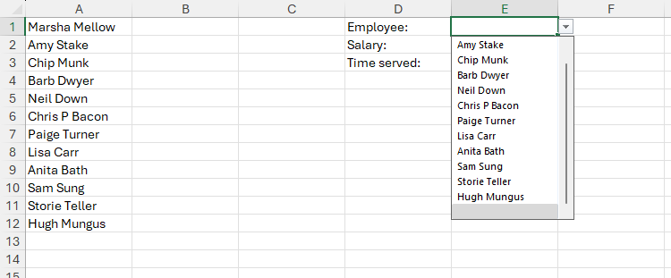
Finally, named ranges are helpful in creating dynamic drop-down lists through Excel’s Data Validation tool. In this example, I’ve renamed the whole of column A “Employee_Names.” Now, when I click “Data Validation” in the Data tab on the ribbon to add a drop-down list of names to cell E1, I can specify the source of my list as this named column.

This means that any names I add to column A will be included in the drop-down list.

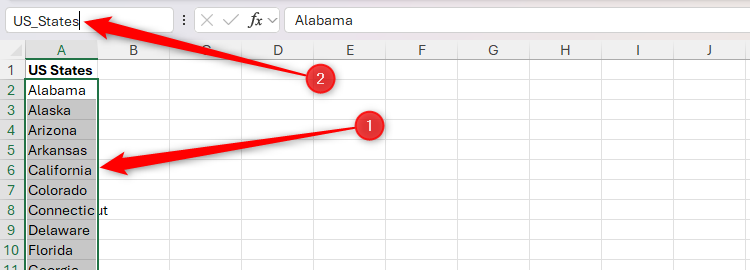
Naming a cell or a range of cells in Excel is straightforward. Simply select the cell or range you want to name, and replace the cell reference with the desired name in the name box. Then, press Enter.

When you use this method to name ranges manually, there are some rules you must follow for Excel to accept your changes:

• The first character must be a letter, underscore (_), or backslash (\).
• The remainder of the name mustn’t contain any special characters. In other words, you can use letters, numbers, periods, and underscores only.
• If the name you assign contains more than one word, use underscores or periods (.) as word separators. You can’t use spaces.
• A named range cannot be the same as a cell reference, like A1 or B$2.
• You can’t call a range “R,” “r,” “C,” or “c,” as these references are reserved for other background uses in Excel.
• Each range name must be different to other names in the workbook, and Excel doesn’t distinguish between upper and lowercase letters.
• Names can be up to 255 characters in length—although this shouldn’t be an issue, as the names you assign should be clear and concise.

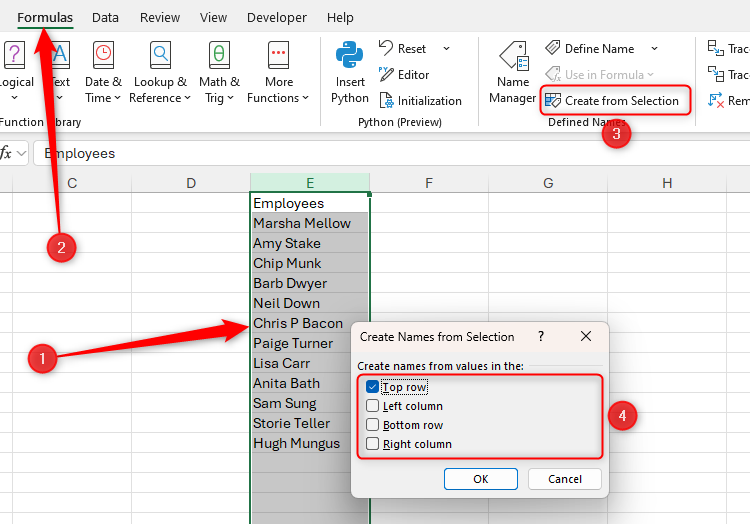
You can also force Excel to name a range based on data you already have in your worksheet. Select the range you want to name, and in the Formulas tab on the ribbon, click “Create From Selection.” Then, check the relevant option in the dialog box that appears. In this example, checking “Top Row” will result in the range being named “Employees,” because the column header is included in the selection.

How to Change a Named Range in Excel

Whether you want to change the name of a range or the cells included within a named range, the process is quick and easy.

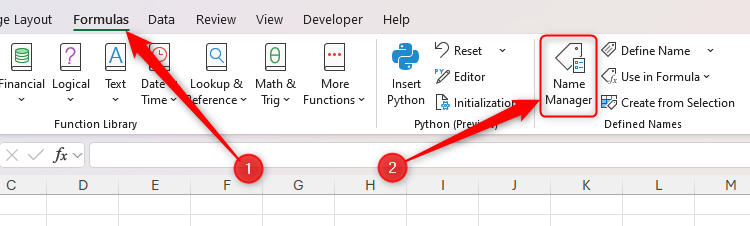
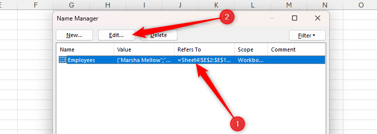
In the Formulas tab on the ribbon, click “Name Manager.”

Then, double-click the named range you want to modify, or single-click it and select “Edit”

Next, in the Edit Name dialog box, you can change the name of the range in the Name field, or adjust the referenced range in the Refers To field.

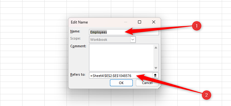
When you’re done, click “OK,” and close the Name Manager dialog box. If you included the previous name or range in a formula, Data Validation condition, or another reference in your workbook, don’t worry—these will update automatically according to the changes you just made.

Before you go ahead and name some ranges in your workbook, here are some points to note:

• Use descriptive but short names. For example, “Total_expenditure_for_the_year_2020” will only serve to make formulas unbearably long and cause confusion. Likewise, “TotExp20” might not provide enough information to someone who hasn’t seen the sheet before. Instead, a name like “Expenditure_2020” would be more suitable.
• Not every range has to be named. Sometimes, unnamed ranges (direct cell references) can be more useful if you share the sheet with others, as they can see the exact reference location. In other words, you should only name ranges when doing so will add value to the spreadsheet.
• You could consider prefixing any named ranges with “Rng_” to distinguish them from other named items, like tables or charts. Taking this step also makes the ranges easier to identify in formulas—when you type Rng, all the named ranges will appear in a tooltip list, and you can simply select the relevant range.
• Another way to name ranges in Excel is to format the data as an Excel table, and rename the table instead.