How Checkboxes Work in Excel

Before I show you how to format a whole Excel row when a checkbox in that row is checked, let’s take a moment to understand how checkboxes work.

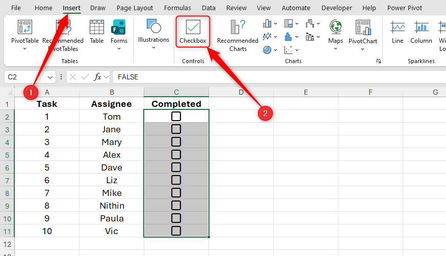
To add checkboxes to selected cells, click “Checkbox” in the Insert tab on the ribbon.

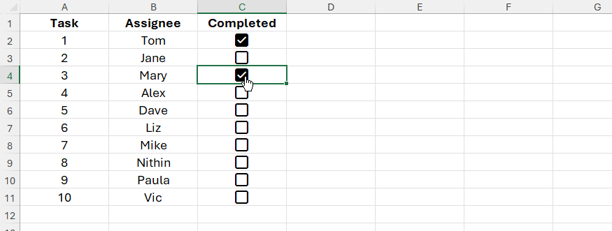
You can manually check and uncheck a checkbox by clicking it or selecting the cell and pressing Space.

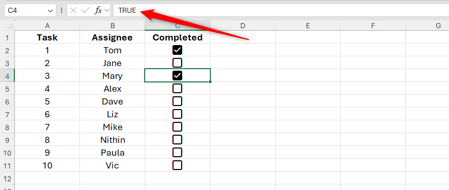
All checkboxes have underlying Boolean values: a checked checkbox represents a value of TRUE, while an unchecked checkbox represents a value of FALSE. You can see this by selecting a cell containing a checkbox and looking in the formula bar. Knowing these underlying values will help you immensely when you go to use checkboxes to format whole rows in Excel.

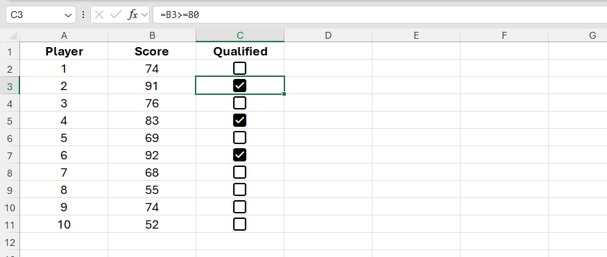
Because checkboxes represent TRUE or FALSE, you can use formulas to check and uncheck them. In this example, the checkbox in cell C3 is checked because the value in cell B3 is greater than or equal to 80.

Formatting Whole Rows in Regular Ranges When a Checkbox Is Checked

Now that you know how checkboxes work, you’re ready to use them alongside conditional formatting to format a whole row.

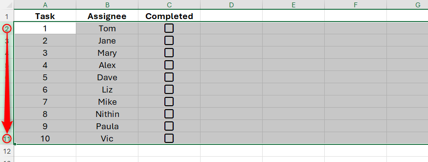
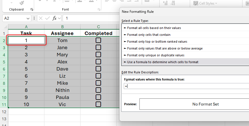
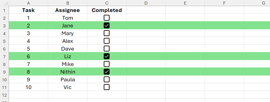
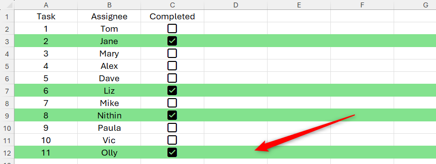
Suppose you’ve created this spreadsheet, which contains task numbers in column A, assignees in column B, and checkboxes in column C, all in a regular Excel range (in other words, not formatted as an Excel table).

Your aim is to format a whole row when a task is completed. That is to say, when you check a checkbox in column C, you want the whole row that the checkbox is on to adopt certain formatting.

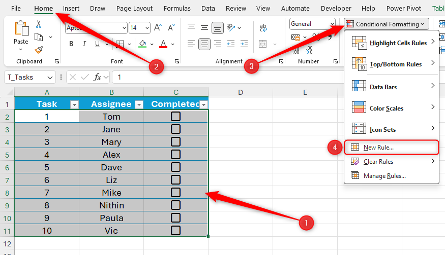
To do this, first, select rows 2 to 11 by clicking and dragging the cursor from the row heading of row 2 to the row heading of row 11.

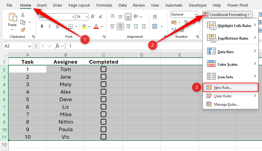
Next, in the Home tab on the ribbon, click Conditional Formatting > New Rule.

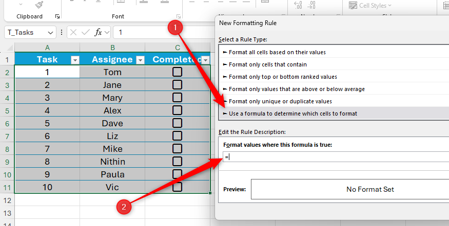
Then, in the New Formatting Rule dialog box, click “Use A Formula To Determine Which Cells To Format.”

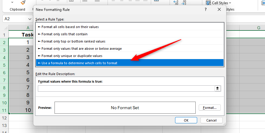
The reason you need to use a formula is that the formatting of the selected rows is dependent on the value of another cell. In this case, you want the row to be formatted when the corresponding checkbox in column C is checked (thus representing the Boolean value TRUE). On the other hand, if the checkbox is unchecked (thus representing the Boolean value FALSE), the formatting of the respective row will remain as is.

So, in the formula field, start by typing an equal (=) sign.

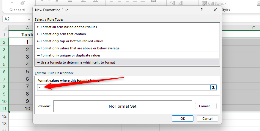
When applying conditional formatting rules to a range of cells in Excel, the formula you type must correspond to the first cell you selected. You can tell which cell was the first one you selected by seeing which one in the selection is white. In this case, because the first row you selected was row 2, you need to focus on creating a rule that applies to this row.

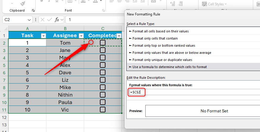
As a result, since you want to check whether the checkbox cell C2 is checked, select this cell to add a reference to the formula.

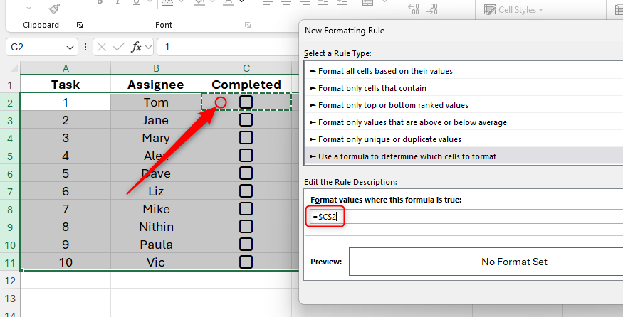
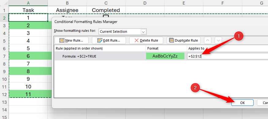
Notice how, at the moment, the cell reference contains a dollar sign before both the column and row, also known as an absolute reference. This means that all the rows you selected will be formatted when the checkbox in cell C2 is checked. However, this isn’t what you want—you only want row 2 to adopt the formatting. So, with your cursor placed directly after the $C$2 cell reference in the formula, press F4 twice, so that only the column reference is preceded by a dollar sign.

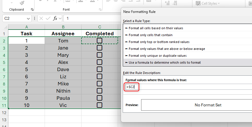
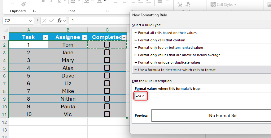
Now, the column reference is absolute, but the row reference is relative, meaning that the rule will adapt to each row. In other words, the reference for row 3 will be $C3, the reference for row 4 will be $C4, and so on.

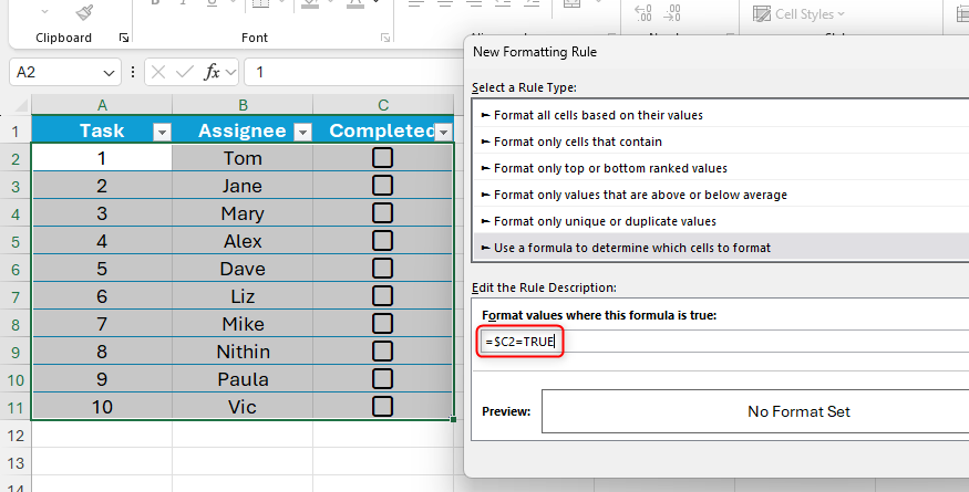
Next, you want to complete the formula by evaluating whether the checkbox is checked. To do this, type another equal sign, followed by TRUE:

=$C2=TRUE

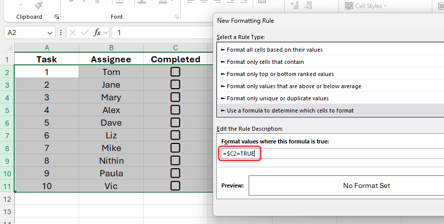
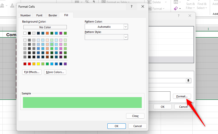
Then, click “Format,” and choose the formatting you want to apply when the rule is fulfilled. In my case, I want the whole row to turn green, but you can also apply other formatting via the Font tab, like turning the font red or using a strikethrough effect.

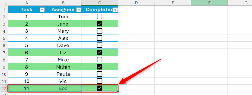
Finally, click “OK” twice to close the two dialog boxes, and check one of the checkboxes to see your new rule in action.

Pros and Cons of Using Conditional Formatting to Format Whole Rows in Regular Ranges

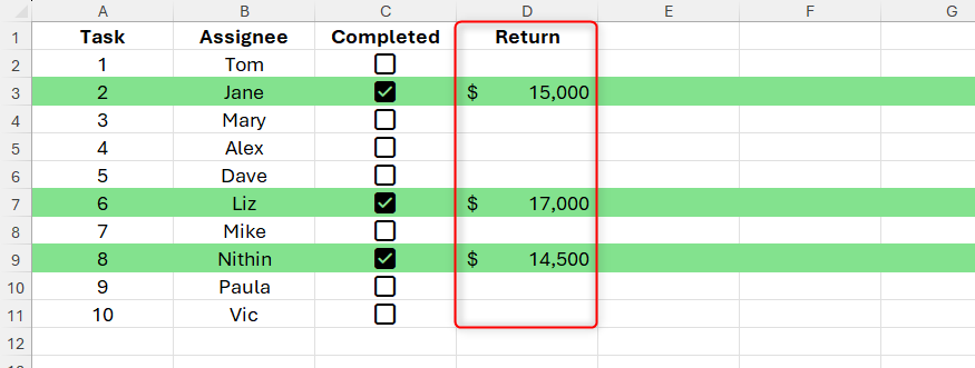
One of the benefits of formatting a whole row is that if you add more data to the right, the rules you set up already apply to these additional columns, so there’s no extra work for you to do.

However, this approach also comes with two significant drawbacks. First, formatting whole rows can significantly hamper Excel’s performance. This is especially true when you apply formatting through conditional formatting because it constantly re-evaluates whenever the data is changed. To overcome this, rather than selecting whole rows, apply the conditional formatting rule to the range width only.

The second drawback becomes evident when you populate rows directly beneath the range. When you do this, Excel generates inaccurate conditional formatting rules as it struggles to account for the changes in the size of your data.

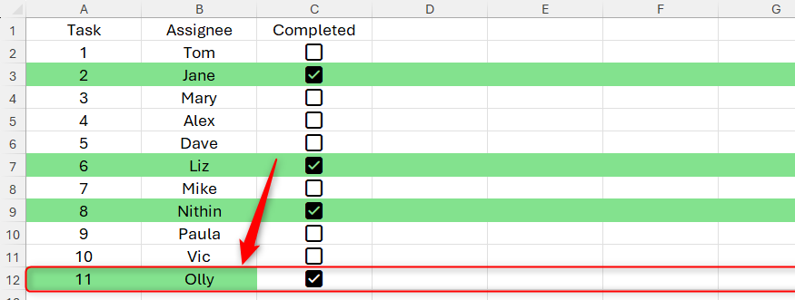
To fix this, select any cell containing the correct rule you set up earlier, click Conditional Formatting > Manage Rules in the Home tab, and expand the cell reference in the Applies To field by one row. For example, if the rule currently applies to rows 2 to 11, change “11” to 12, and click “OK.”

This tweak to the rule now picks up the extra row of data and formats it accordingly.

Formatting Whole Rows in Excel Tables When a Checkbox Is Checked

If, like me, you prefer presenting your data in Excel tables rather than using unformatted ranges, you can format a whole table row when a checkbox is checked.

After adding the checkboxes via the Insert tab on the ribbon, select the whole table—starting in cell A2 and finishing in cell C11—and in the Home tab on the ribbon, click Conditional Formatting > New Rule.

Now, click “Use A Formula To Determine Which Cells to Format,” and begin the formula in the text field with an equal sign.

Since cell A2 is the active cell in the selection, you need to generate a formula that applies to row 2. So, select the cell on row 2 that contains the checkbox (in this case, cell C2) to add a reference to the formula.

The cell reference is currently absolute, meaning all the cells in the table will be formatted when the checkbox in cell C2 is checked. To fix this, press F4 twice, turning it into a mixed reference where the column is fixed and the row is relative.

Now, complete the formula by typing another equal sign, followed by TRUE, to tell Excel that you only want to format the rows where the corresponding cell in column C contains TRUE (a checked checkbox).

Finally, click “Format” to apply the relevant formatting, and then click “OK” twice to close the dialog boxes and see the rule working in your dataset.

Pros and Cons of Using Conditional Formatting to Format Table Rows

One of the biggest benefits of using Excel tables is that new rows added to the bottom of the existing dataset adopt the rules and formulas applied to the rows above. As a result, you can easily expand your data downward without worrying about tweaking the conditional formatting rule you just created.

Another benefit of formatting a table row rather than the whole row in the spreadsheet is that you’re not asking Excel to work as hard. In the example above, checking a checkbox only applies formatting to three cells, rather than the 16,000-plus cells that make up the width of an Excel spreadsheet.

That said, a drawback of using conditional formatting to format table rows is that the rule doesn’t apply to new columns added to the right.

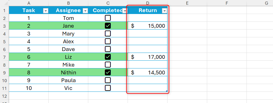
To fix this, select any cell containing the rule you set up earlier, click Conditional Formatting > Manage Rules in the Home tab, and expand the cell reference in the Applies To field by one column. For example, if the rule currently applies to columns A to C, change “C” to D, and click “OK.”

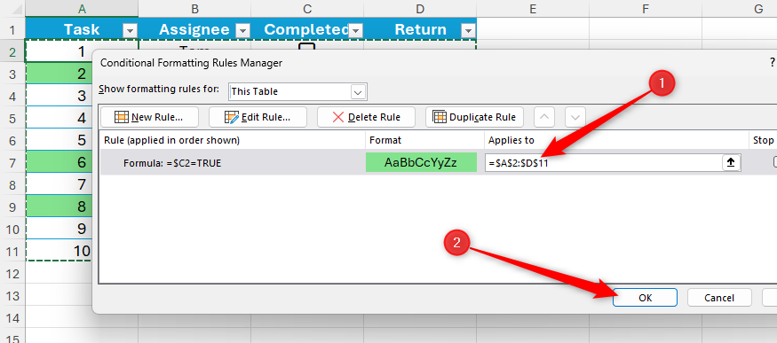
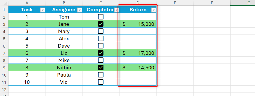
Now, the new column adopts the whole-row conditional formatting.