Situatie
Solutie
Think of LAMBDA as a custom formula you write on the fly—instead of a fixed cell reference like A2*0.15, you define a parameter:
=LAMBDA(x,x*0.15)
where:
- x is the parameter that represents the value the function will process.
- x*0.15 is the calculation you want Excel to perform on that parameter.
On its own, this formula doesn’t do much; it needs a driver to take that logic and apply it to your data. That’s where the LAMBDA helper functions come into play.
Excel tables don’t support spilled results. If you try to place a dynamic array formula like MAP or SCAN inside one, you’ll trigger a #SPILL! error. To avoid this, always place your LAMBDA helper functions in the standard grid.
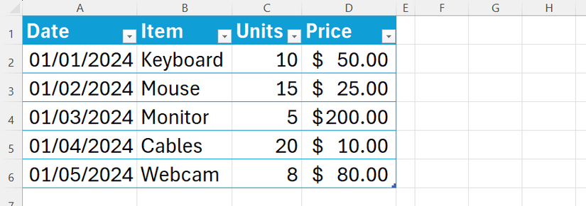
In this run-through, I’ll use the following table—named T_Gadgets—as the data source and enter the formulas in regular cells next to or above it.
The iterators (MAP, BYROW, BYCOL): Applying logic to every cell, row, or column
Iterators walk through your table data and apply LAMBDA logic to each item.
MAP: Apply logic to every single cell
| The syntax | =MAP(array,LAMBDA(parameter,calculation)) |
|---|---|
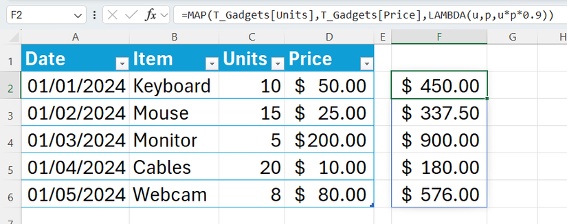
| The aim | You want to calculate the revenue for each row in T_Gadgets and apply a 10% discount at the same time. |
| The benefit | The entire calculation lives in one place. This makes your logic more secure, as individual rows within the results can’t be overwritten. |
Here’s the MAP formula you need to type into cell F2:
=MAP(T_Gadgets[Units],T_Gadgets[Price],LAMBDA(u,p,u*p*0.9))
where:
Use MAP to combine parallel columns; use BYROW (below) to treat each record as a single bundle of data.
BYROW: Get a result for every row
| The syntax | =BYROW(array,LAMBDA(row,calculation)) |
|---|---|
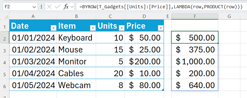
| The aim | You want to multiply the Units and Price in T_Gadgets horizontally to get the total revenue for each row (day). |
| The benefit | Instead of managing formulas across hundreds of rows, you manage one formula in a single cell that spills down, ensuring consistency across your dataset. |
The BYROW formula for cell F2 is as follows:
=BYROW(T_Gadgets[[Units]:[Price]],LAMBDA(row,PRODUCT(row)))
where:
- Array: T_Gadgets[[Units]:[Price]] is the range encompassing both columns.
- Parameter: row represents an entire horizontal row of data.
- Calculation: PRODUCT(row) multiplies every value found within that row.
BYCOL: Get a result for every column
| The syntax | =BYCOL(array,LAMBDA(column,calculation)) |
|---|---|
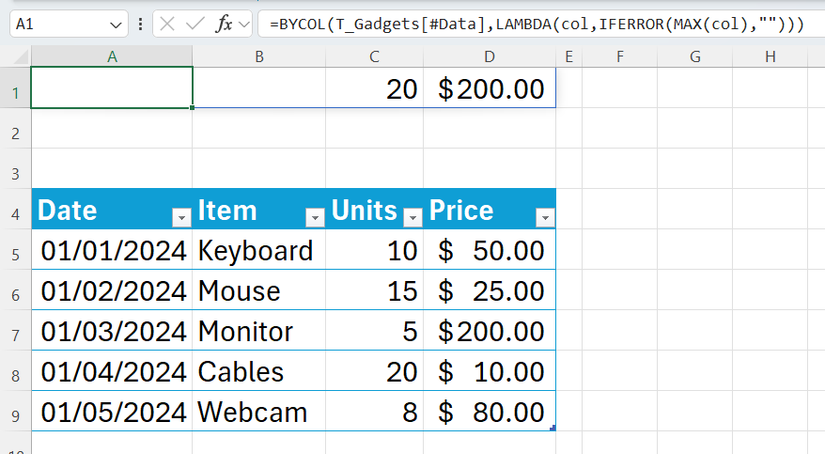
| The aim | You want a single formula that finds the maximum value for the Units and Price columns in T_Gadgets. |
| The benefit | By using BYCOL in a row above the table, you create a header summary. This saves you from having to scroll down to a Total Row at the bottom of a massive table, and condenses the logic into a single cell for security and consistency. |
Here’s the BYCOL formula for cell A1:
=BYCOL(T_Gadgets[#Data],LAMBDA(col,IFERROR(MAX(col),"")))
where:
Functions like MAX and SUM will often return 0 for a text column. To hide this value without breaking the formula’s alignment, select the cell containing the zero, and in the Format Cells dialog (Ctrl+1), use the custom number format ;;; (three semicolons) to make the value invisible while keeping the cell functional.
The accumulators (SCAN and REDUCE): Building results as you go
Accumulators have memory, keeping a running tally as they move through your table.
SCAN: Create a running total or running count
| The syntax | =SCAN(initial_value,array,LAMBDA(accumulator,value,calculation)) |
|---|---|
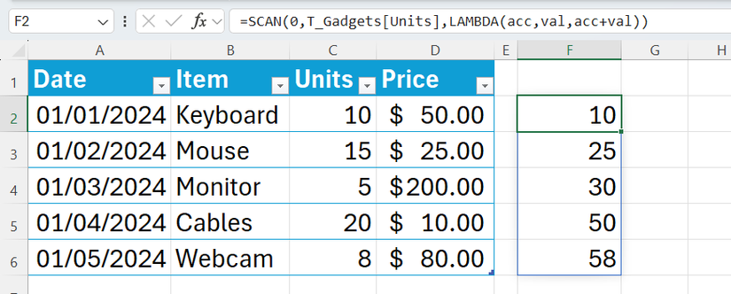
| The aim | You want to see a daily running total of the Units column in T_Gadgets to track inventory depletion. |
| The benefit | Traditional running totals like =SUM($C$2:C2) can break if you sort or delete a row. SCAN keeps the logic in one cell, making it immune to structural changes. |
In this example, the SCAN formula for cell F2 is as follows:
=SCAN(0,T_Gadgets[Units],LAMBDA(acc,val,acc+val))
where:
- Initial value: 0 is where the count starts.
- Array: T_Gadgets[Units] is the column you’re scanning.
- Parameters: acc,val are the parameters—the accumulator that memorizes the previous total, and the value of the current cell being added to the memory.
- Calculation: acc+val is the logic that updates the memory.
REDUCE: Shrink an array into one final value
| The syntax | =REDUCE(initial_value,array,LAMBDA(accumulator,value,calculation)) |
|---|---|
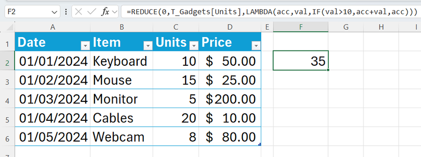
| The aim | You want to sum the Units in T_Gadgets, but only for bulk orders (sales of more than 10 items). |
| The benefit | REDUCE condenses multistep logic into a single cell, avoiding nested SUMIFs, helper columns, or multiple intermediate steps. |
In cell F2, type this REDUCE formula:
=REDUCE(0,T_Gadgets[Units],LAMBDA(acc,val,IF(val>10,acc+val,acc)))
where:
- Initial value: 0 is the starting point for your sum.
- Array: T_Gadgets[Units] is the column being reduced.
- Parameters: acc,val are the parameters—the final accumulated result being built as the function runs, and the value of the current cell being added to the accumulation.
- Calculation: IF(val>10,acc+val,acc) adds the value to the total only if it’s over 10.
Leave A Comment?