The Python statistics module is a built-in module for performing simple statistical calculations. Since it’s part of the standard Python library, it’s available in every Python installation. To access it in scripts or interactive sessions, all you have to do is import it:

import statistics

If you need just one or a few functions from a Python module in an interactive session, such as in IPython or a Jupyter notebook, you can import them directly into the current namespace, so you don’t have to type out “statistics” all the time. This is what the examples in this article will assume.

The statistics module shines in an interactive Python mode like the interpreter, an enhanced session in IPython, or a Jupyter notebook.

Descriptive Statistics

The most basic form of statistics is descriptive statistics. As the name implies, these statistics are intended to describe the data, such as its central tendencies or measures of dispersion.

The simplest calculation is the arithmetic mean, which is just the sum of the data points divided by the number of data points. In statistics textbooks, the sample mean is represented by an x with a bar drawn over it, known as “x-bar.” The population mean is represented by the Greek letter, mu, but it’s the same calculation. Most people will know this as the “average”.

To calculate the mean with the statistics module, just use the mean function.

Only import functions into the main Python namespace in interactive sessions. Doing this can cause bugs in scripts if the imported function overrides a built-in function.

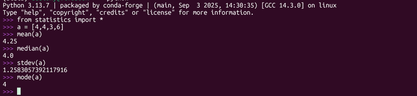
Let’s create a small array of numbers and find the mean:

a = [4,4, 3, 6]
mean(a)

The result is 4.6.

The fmean function also computes means, but converts the data to floating-point numbers. It will also let you compute a weighted mean.

weights = [1,2,3,4]
fmean(a,weights)

The weighted mean from this example is 4.5

Another kind of mean is the geometric mean, which is useful for comparing growth rates over a period of time. It involves taking the nth root of the data points multiplied together. By hand, this usually means tedious logarithms, but it’s easy in Python with the geometric_mean function.

geometric_mean(a)

The harmonic mean is the reciprocal of the arithmetic mean. Its the number of data points divided by the sum of the fraction of 1 / the first data point, 1 / the second data point, and so on. The harmonic mean is useful for taking averages of things like speeds that have certain rates. Fortunately, Python can also do this for you.

harmonic_mean(a)

The result is 4. Notice that the harmonic mean was less than the geometric mean, and the geometric mean was less than the arithmetic mean on the same set of data.

The median is another popular measure of central tendency. It’s the data point that divides a data set in half. You can find it with the median function:

median(a)

The result is 4 in our sample.

The mode function reports the most common number in the sample.

mode(a)

Again, the mode is 4, since it’s the most common recurring number in the array we defined earlier.

Another common reason for taking descriptive statistics is to measure of spread of the data, also known as dispersion. The best known measure of spread is the standard deviation, which measures how far the data are spread out from the arithmetic mean. It’s the square root of the variance, or the sum of the square of the mean subtracted from each data point, divided by the number of data points. This represents the population standard deviation, but the standard deviation subtracts the number of data points by one to give a more representative result in smaller samples.

The stdev function computes the sample standard deviation, which will likely be what you want most of the time:

stdev(a)

The result is approximately 1.26.

Let’s compare it to the population standard deviation with the pstdev function:

pstdev(a)

You can view the sample variance with the variance function

variance(a)

It also has a population-based variant, pvariance, that works the same way.

Another way to view the distribution of your data is to divide it into percentiles, which the percentage of data points that are less of that. The median is actually the 50th percentile, since half of the data points are below.

The quantiles function will divide the data into percentiles by result:

quantiles(a)

It will show the lower quartile, or 25th percentile, the median, and the upper quartile. The built-in min and max functions will display the minimum and maximum values.

min(a)
max(a)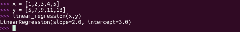

Regression and Correlation

A popular statistical method is to see how one variable is correlated with another. This amounts to plotting data points on x-and-y axes and drawing a line over them to see how well it fits. This is known as “linear regression.” The statistics module has a method for simple linear regression. It’s “simple” because it only correlates two variables. It uses a method called “ordinary least squares,” so called because it tries to minimize the square of the distance between the data points and the line it creates.

Let’s plot a linear regression of two arrays labeled x and y

x = [1,2,3,4,5]
y = [5,7,9,11,13]

To fit the model, use the linear_regression method. This will calculate the slope and the y-intercept for the familiar equation of a line: y = mx + b.

linear_regression(x,y)

This will give you the slope and the intercept. You can also save them in variables:

slope, intercept = linear_regression(x,y)

The slope in this case is 2, and the intercept is 3, representing the slope-intercept equation y = 2*x + 3. The positive sign on the slope indicates that it’s an upward-sloping line, which means that the y value will increase as we move to the right.

This function won’t plot any lines or the classic scatterplot. It will also only give you the regression for two variables. If you want to generate a plot or make a prediction using more than one dependent variable, you’ll have to use other libraries such as Seaborn, statsmodels, or Pingouin.

You can see how well two variables correlate using the correlation function. This calculates the correlation coefficient, or r. This coefficient will be between 0 and 1 or -1, indicated a positive or negative correlation. A negative correlation will mean a downward-sloping line.

Two check the correlation between two variables:

correlation(x,y)

In this case, it’s 1, showing a perfect positive correlation, but real data rarely correlates this perfectly. This means that the regression line will lie perfectly on the data points when you plot them.

The Normal Distribution

The normal distribution, with its famous bell-shaped curve, is a continuous probability distribution. You can use the function to estimate the probability of some normally distributed parameter.

We can demonstrate this with data from the CDC. According to the data, the mean of males over 20 is 175.1 centimeters. We can get the population standard deviation by multiplying the square root of the number of samples, 2,690, by the standard error, .3

import math
math.sqrt(2690) * .3

The standard deviation is approximately 15.56

We can use this to build a normal distribution object:

men_height = NormalDist(175.1,28.41)

To find the percentage of men who are between 160 and 180 centimeters tall, we use the cumulative distribution function, or CDF, which gives the percentage of values of a simple below a certain value. We can subtract the lower value from the higher one because the normal distribution curve is symmetrical. The object we just created has a cdf method we can use to give us this probability.

men_height.cdf(180) - men_height.cdf(160)

The answer will be that approximately 45% of men are between 160 and 180 centimeters tall.

NumPy, SciPy, and other libraries are popular for statistics and data analysis. Where does that leave the statistics module? The former libraries are designed for large data sets and professional use. The developers of the statistics modules have pitched it at the levels of scientific and graphing calculators. This library is fine for learning statistical concepts and quick, casual calculations.

If you want to work with real datasets, the other libraries are going to be more powerful and flexible, although the learning curve can be steep. If you want a taste of the power of statistical computing with Python, the statistics module is a good place to start.