Before I show you a real-life example of SWITCH in action, let’s look at the syntax:

=SWITCH(e,v1,r1,v2,r2,d)

where

• e is the expression (the value that will be evaluated),
• v1 is the first value to be compared against the expression,
• r1 is the result that will be returned if v1 matches e,
• v2 is the second value to be compared against the expression,
• r2 is the result that will be returned if v2 matches e, and
• d (optional) is the default value if e does not match any of the v values.

While there are only two v–r pairings shown here in the syntax (v1–r1 and v2–r2), you can have up to 126 pairings overall. Given that SWITCH returns a result corresponding to the first matching value, it’s important to carefully consider the order of your v–r pairings.

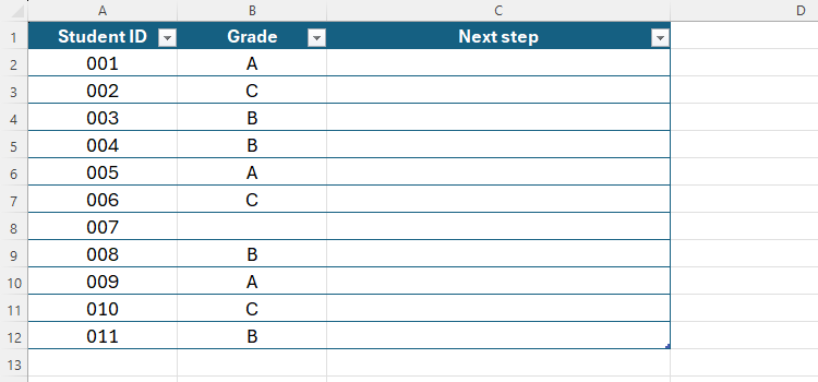
Let me show you the SWITCH function in a real-world scenario. In this table, I have a list of students and their grades, and I need to work out their next steps based on those grades.

Since there are three different grade possibilities (A, B, and C), I need to incorporate all of these into the SWITCH formula. So, in cell C2, I will type

=SWITCH([@Grade],"A","Automatically advance to next level","B","Continue at this level","C","Move down to previous level","GRADE REQUIRED")

Although this looks complicated at first, when broken down, it’s actually quite logical:

• First, I want Excel to evaluate the expressions in the Grade column of my formatted table, which is why I typed [@Grade] as value e.
• Then, I have three v–r pairings: “A” will return “Automatically advance to next level,” “B” will return “Continue at this level,” and “C” will return “Move down to previous level.”
• Finally, after the final pairing, I have stated “GRADE REQUIRED” as value d, which is the result if none of the values (v#) matches the expression (e).

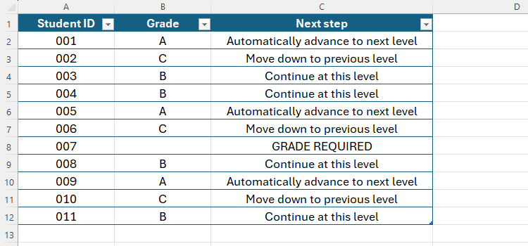
After pressing Enter, because my data is in a formated Excel table, the rest of column C will populate automatically.

Notice how cell C8 contains “GRADE REQUIRED,” because the expression in cell B8 did not match any of the values in my SWITCH formula.

You may be wondering why you would use SWITCH over some of Excel’s other functions that perform similar actions, such as IF, IFS, and XLOOKUP. Here are some reasons:

Avoid Repeating the Expression

To create the same results in the table above using IF or IFS, I would have to repeat the expression each time:

=IFS([@Grade]="A","Automatically advance to next level",[@Grade]="B","Continue at this level",[@Grade]="C","Move down to previous level")

With the SWITCH function, however, I only have to state the expression once at the start of the formula:

=SWITCH([@Grade],"A","Automatically advance to next level","B","Continue at this level","C","Move down to previous level","GRADE REQUIRED")

As a result, the SWITCH function is easier to read, less prone to typing errors, and easier to review if there’s an issue.

Keep Everything in One Place

Much like SWITCH, the XLOOKUP function compares an expression to a list of values, and returns a corresponding value. However, with XLOOKUP, the list of values is in a separate table, whereas SWITCH incorporates them all into one formula. This means that you don’t have any floating data, and so, your Excel spreadsheet stays tidy.

One Set of Parentheses

If I chose to use nested IF functions to achieve the same outcomes in the table above, I would have had to use a new set of parentheses for each IF argument:

=IF([@Grade]="A","Automatically advance to next level",IF([@Grade]="B","Continue at this level",IF([@Grade]="C","Move down to previous level","GRADE REQUIRED")))

As a result, the formula ends confusingly with three closing parentheses, and debugging any issues with the syntax would be more challenging. On the other hand, when used at its most basic level without any other additional functions, SWITCH requires only one pair of parentheses.

SWITCH Drawbacks

While SWITCH has many benefits, there are a few limitations to bear in mind before you get working on your Excel spreadsheet:

• You can’t use operators (such as < or >) or approximate matches with the standard SWITCH syntax. Instead, SWITCH is limited to exact matching only.
• If you have lots of potential values and results, constructing your SWITCH formula in the first instance will take forever. Personally, I would recommend using no more than seven or eight value-result pairings in your SWITCH formula.
• SWITCH is a relatively inflexible function. For example, XLOOKUP can return entire rows and columns of data, rather than just a single value.
• Because SWITCH requires lots of commas (and quotes if you’re including non-numerical values), it’s easy to make a mistake if you type the formula manually.