Situatie
Solutie
Conditional formatting is a trap
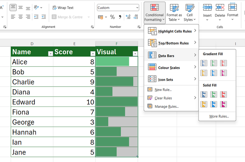
However, as your workbook grows from a few dozen rows to a few thousand, the cracks start to show. The biggest issue with data bars isn’t the formatting itself—it’s how Excel manages it. Copying and pasting ranges with conditional formatting can sometimes create duplicate rules or misaligned ranges, requiring manual cleanup. There’s also the lag factor. Data bars recalculate whenever their source data changes, which can impact performance in very large datasets with frequent updates.
Excel treats the REPT output as simple text, making it significantly more lightweight and stable than graphical rendering.
The REPT function is the way forward
Excel’s REPT function is one of Excel’s simplest tools, usually tucked away for basic text manipulation. Its syntax is straightforward:
=REPT(text,number_of_times)
Simply choose a character, and use a number, cell reference, or formula to tell Excel how many times to repeat it. Before you know it, you’ve created a bar that lives directly inside the cell as text.
Always use formatted Excel tables (Ctrl+T) to ensure your formulas bleed down into new rows as you add data. The default table style in Excel uses banded rows, which can diminish the impact of your visuals, so after creating your table, open the “Table Design” tab and choose a plain style.
Before you ditch conditional formatting entirely, it’s worth noting that Excel’s built-in data bars offer a few premium features that the REPT function can’t replicate alone, like gradient fills and the ability to grow to the left for negative numbers. However, as I explained above, by choosing the REPT function, you’re prioritizing stability and performance over visual finesse.
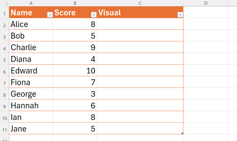
Example 1: The basic bar
Imagine you’re a manager tracking team performance scores on a simple scale of 1 to 10.
First, select the column where your data bars will go, and change the font to Playbill or Britannic Bold (these squish the individual characters into a solid bar without spaces). Then, in the top cell of the column, insert this formula and press Enter:
=REPT("|",[@[Score]]*5)
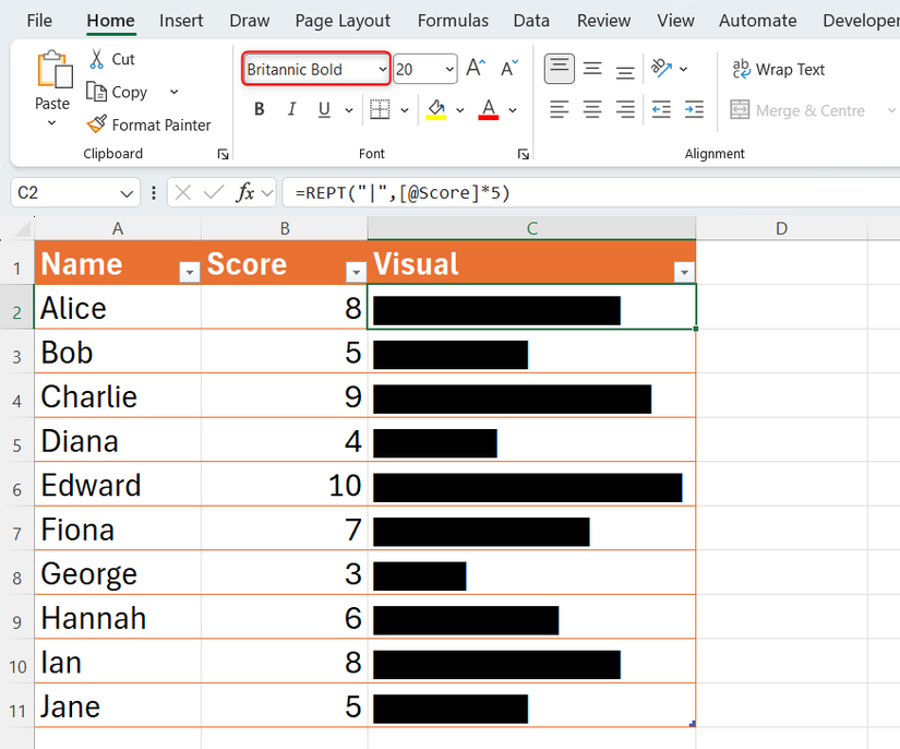
On standard U.S. keyboards, the pipe character (|) is paired with the backslash (\) and requires you to hold Shift. On other keyboards, it’s next to the Z or Enter key.
Example 2: Relative scaling
Now, suppose you’re analyzing regional sales figures that range from the hundreds to the thousands.
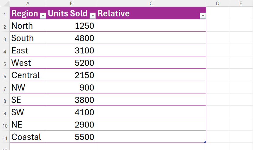
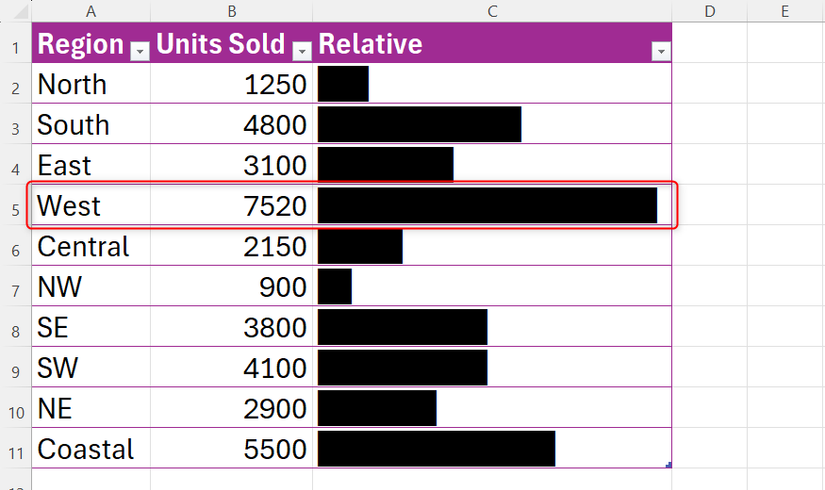
To mimic how Excel’s built-in data bars grow and shrink relative to other values in the range, you need to normalize your data using the MAX function. This prevents a value of 5,000 from being rendered as 5,000 individual characters in a single cell.
Change the font in the visualized column to Consolas. Then, enter this formula and press Enter:
=REPT(UNICHAR(9608),([@[Units Sold]]/MAX([Units Sold]))*20)
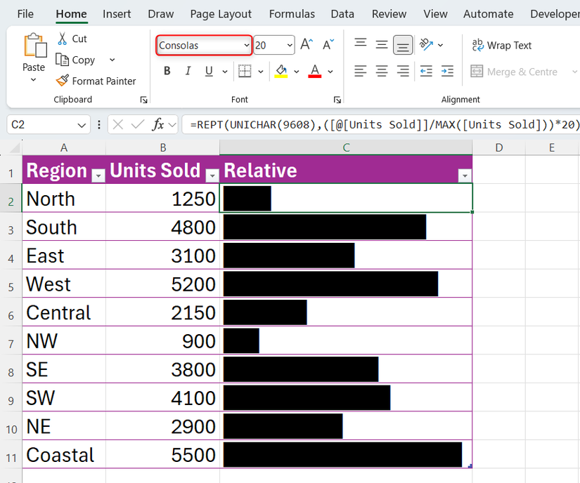
Here’s how the formula works:
| Formula segment | Explanation |
|---|---|
| UNICHAR(9608) | This creates the full block character (█), which is a solid rectangle that occupies the entire width and height of the character space. When entered using the monospaced Consolas font, it’s the perfect building block for a bar that looks like a custom UI element. Using the UNICHAR code ensures the formula works in all versions of Excel. |
| ([@[Units Sold]]/MAX([Units Sold]) | This creates a percentage. If your top salesperson sold 5,000 units and the current row is 2,500, the result is 0.5. |
| *20 | You then multiply the percentage by 20 to tell Excel that the 100% bar should be exactly 20 characters long. |
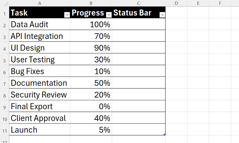
Example 3: The progress tracker
In this third example, let’s assume you’re tracking a software launch and want a “loading bar” that shows both completed work and the work still to be done. While a simple bar shows progress, a dual-character bar provides much more context and looks more professional.
Set the font for your visual column to Consolas, type this formula, and press Enter:
=REPT(UNICHAR(9608),ROUND([@Progress]*10,0))
&
REPT(UNICHAR(9617),10-ROUND([@Progress]*10,0))
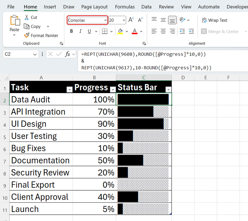
Press Alt+Enter to split long formulas onto separate lines as you type. This makes the formula easier to construct, read, and edit.
Here’s what’s happening:
Example 4: The star rating system
Imagine you’re building a summary sheet for e-commerce product reviews.
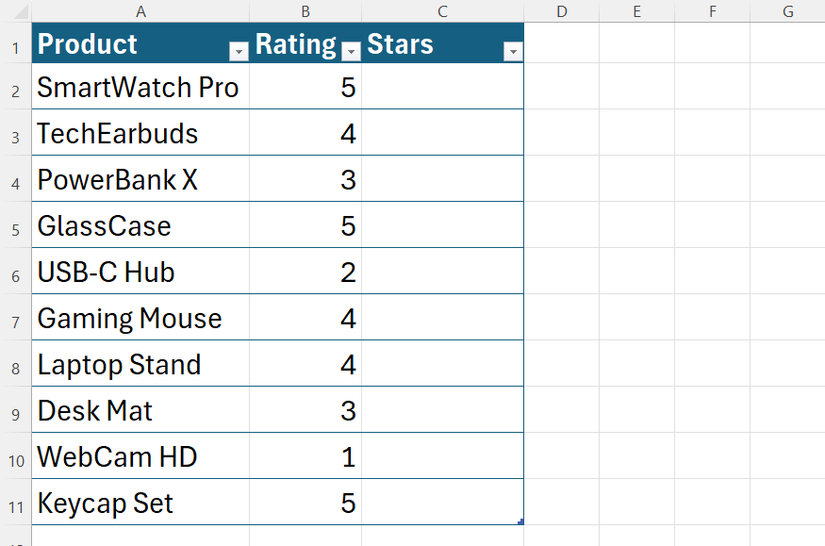
=REPT(UNICHAR(9733),[@Rating])
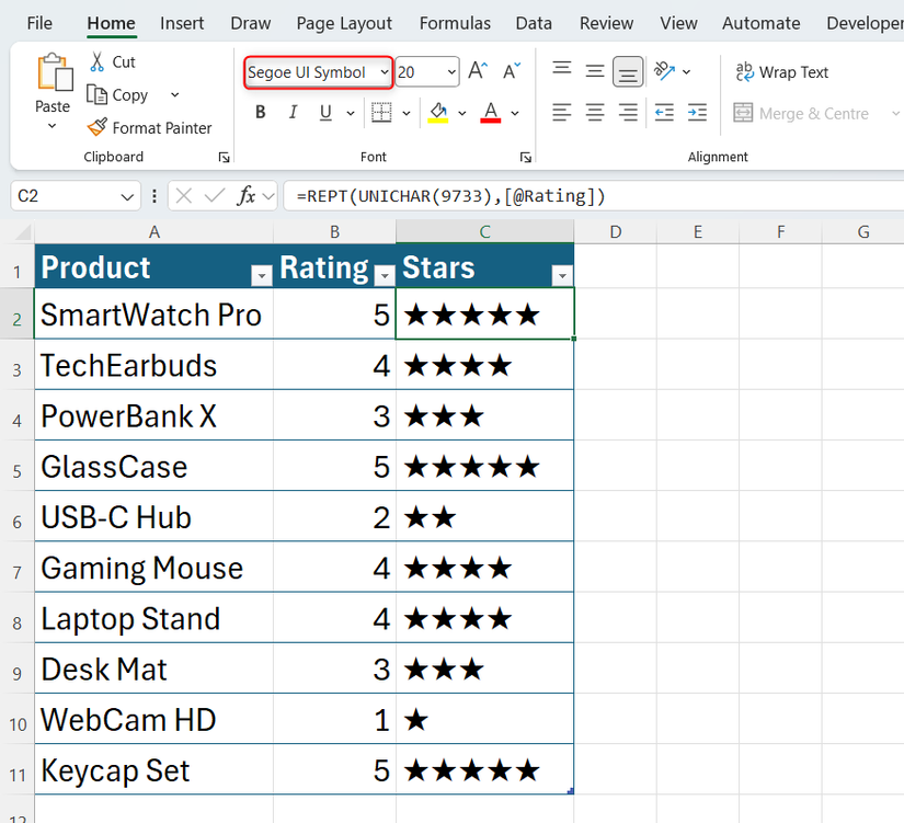
This formula uses REPT in its simplest form: it specifies a Unicode character and uses the values in the Rating column to tell Excel how many times to repeat it. You could also swap the star Unicode character for other codes that better match your data. For example, UNICHAR(9679) creates a modern dot plot (•), and UNICHAR(9670) creates a diamond (♦).
Leave A Comment?