The Camera tool: Capture dynamic snapshots of your data

The Excel ribbon is packed with visual tools, but one of its most versatile layout features is hidden away in the Quick Access Toolbar (QAT) customization menu. The Camera tool lets you take a live, linked snapshot of a cell range (including anything displayed within it) and place it anywhere else in your workbook. Unlike a normal copy-and-paste, the image updates automatically whenever the source data changes.

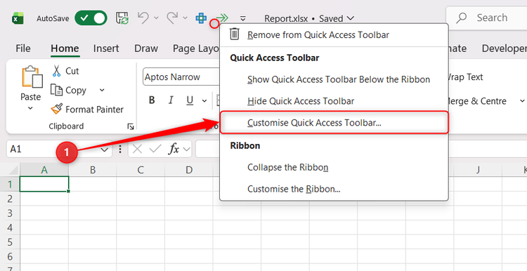
Right-click anywhere on the Excel ribbon, and if you see Show Quick Access Toolbar, click it. If you don’t see this option, it’s already activated. Then, to enable the Camera tool:

1. Right-click the QAT and choose Customize Quick Access Toolbar
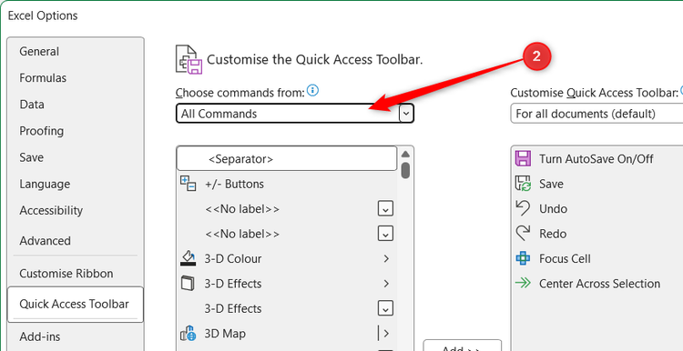
2. Switch the command list to All Commands
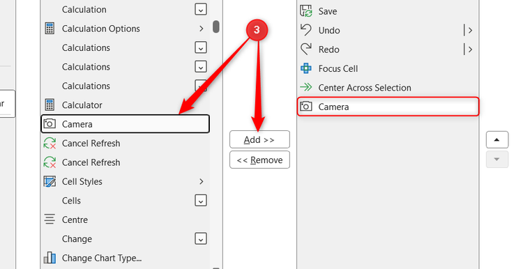
3. Scroll to Camera, select it, and click Add

After clicking OK, you’ll see the Camera icon in your QAT.

Now, select a range of cells and click the Camera icon to create a movable snapshot. Excel then lets you “draw” the image, and the result behaves like a dynamic picture tied directly to the source data. This becomes especially useful when building dashboards or summaries—you can position live snapshots anywhere within the workbook and resize them independently.

Merge & Center is one of Excel’s most deceptively dangerous buttons. It looks harmless enough: you select several cells, merge them into one large cell, and center them across your spreadsheet. The problem is that merged cells interfere with sorting, filtering, copying, and formulas.

Fortunately, Excel has a hidden alignment option that creates exactly the same visual effect without damaging your worksheet structure: Center Across Selection.

To use it:

1. Select the cells you want to “merge”
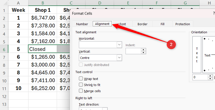
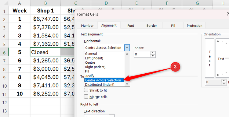
2. Press Ctrl+1 to launch the Format Cells dialog, then open the Alignment tab
3. Expand the Horizontal drop-down menu and select Center Across Selection
4. When you click OK, the text appears perfectly centered across the selected range, but every cell remains independent.

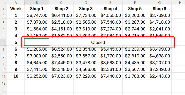
This means your spreadsheet still sorts properly, filters correctly, and behaves normally when referenced in formulas or automation tools. You’ll see the benefit of this when you convert ranges into tables or use them in PivotTables, which don’t always work as expected when merged cells are present.

Proofreading long lists of numbers is exhausting, especially when you’re constantly looking back and forth between a source document and your spreadsheet. Excel’s hidden Speak Cells feature helps reduce that burden by reading your data aloud while you work.

Like the Camera tool, Speak Cells is buried inside the QAT customization menu:

1. Right-click the QAT, then choose Customize Quick Access Toolbar
2. Switch the command list to All Commands
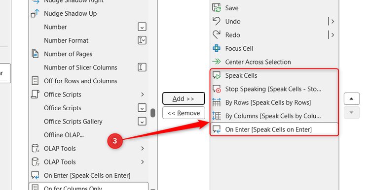
3. Scroll to the following five commands, select them, and click Add:
   1. Speak Cells
   2. Stop Speaking
   3. By Rows (Speak Cells by Rows)
   4. Speak by Columns (Speak Cells by Columns)
   5. On Enter (Speak Cells on Enter)

At first glance, the feature sounds gimmicky, but it becomes genuinely useful in repetitive data-entry workflows. Instead of visually checking every value against a source document, you can keep your eyes on the original while Excel confirms each entry aloud. That reduces the mental overhead of switching your focus, which is often the cause of transcription and checking errors.

Speak Cells can be used in two different ways. You can manually select a range and have Excel read it back as a one-off check (click Speak by Rows or Speak by Columns, then click Speak Cells), or you can click the Speak On Enter icon, which turns it into a real-time validation tool that reads each cell immediately after you confirm an entry with Enter, Tab, or the Arrow keys.

Speak Cells won’t replace proper auditing or validation rules, but it works well as a lightweight, real-time error-checker that quietly catches mistakes before they become a problem.

The “select visible cells” shortcut: Avoid editing hidden data

Manage mixed-visibility data with precision

Few Excel mistakes are more frustrating than working with a range that looks correct, only to realize later that your copy, paste, or formatting action included rows or columns you couldn’t actually see.

When you apply a filter in Excel, hidden rows are automatically excluded from copy operations. However, the real problem arises when you’re working with manually hidden or grouped rows or columns, where Excel still includes data hidden from view.

That’s where the Visible cells only shortcut comes into play. Yes, it’s technically available through the ribbon, but it’s not directly exposed on it—the route is buried several clicks deep, and the Alt-sequence shortcut is lengthy. The fastest way to activate it is with the keyboard shortcut Alt+; (semicolon).

To use it:

1. Select the range with hidden or collapsed rows or columns
2. Press Alt+; to modify the selection to the visible cells only
3. Press Ctrl+C to copy those cells
4. Go to the cell where you want these cells to be duplicated, then press Ctrl+V (or Ctrl+Shift+V to paste values).
5. 

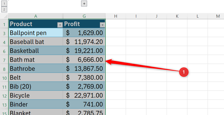
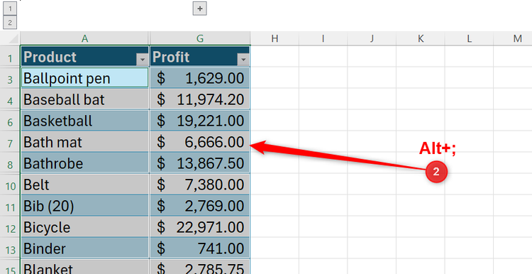
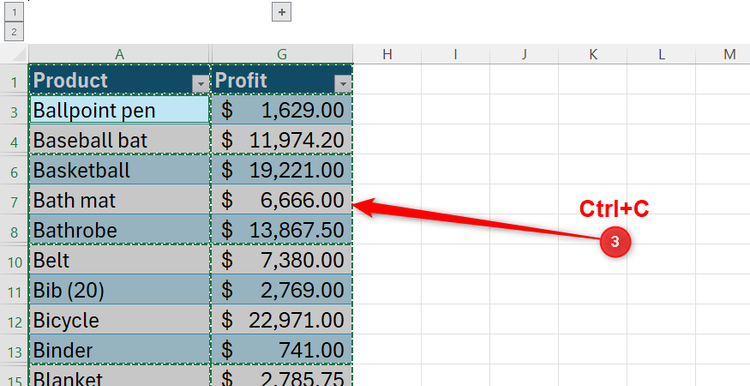
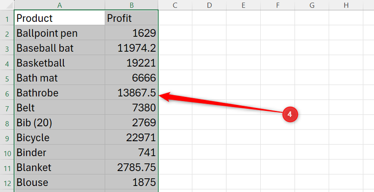
The shortcut becomes especially valuable in large spreadsheets where visibility tools are used constantly. It makes copy-and-paste operations more reliable and helps prevent accidental edits in hidden data, especially during bulk formatting or cleanup passes. Like many advanced Excel habits, this one feels minor at first. After you start using it regularly, though, it quickly becomes part of your normal workflow whenever visibility matters.