Microsoft Excel’s little-known Goal Seek tool is there to help when you know the end goal, but don’t know how to get there.

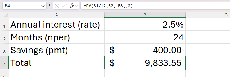
Let’s say you plan to buy a new home in two years’ time. Currently, you’re saving $400 monthly at an annual interest rate of 2.5%, meaning over the two years, you’ll save $9833.55, as calculated through the Future Value (FV) function:

=FV(B1/12,B2,-B3)

where B1/12 turns the annual interest rate (rate, cell B1) into a monthly interest rate, B2 is the number of payments (nper), and B3 is the payment value (pmt) stated as a negative number (since it’s leaving your regular account).

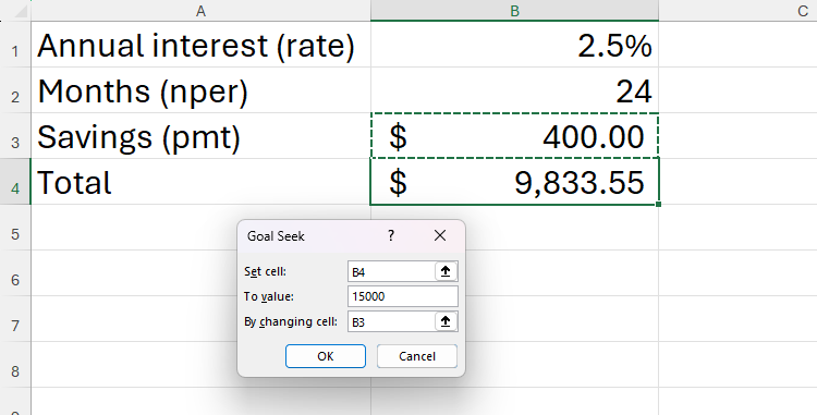
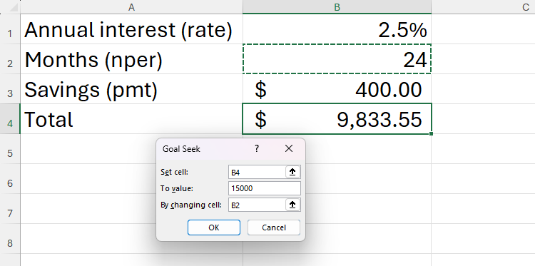
However, you aim to raise a total of $15,000 to cover the cost of the deposit and other expenses that inevitably come with moving house, so you need to work out how much you must save per month over two years to achieve this goal. This is where Excel’s Goal Seek tool comes into play.

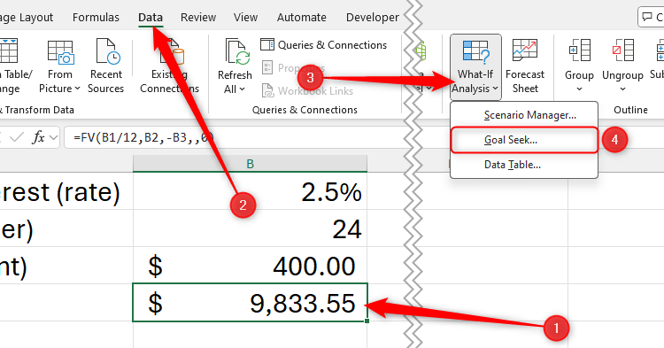
First, select the cell containing the calculation (in this case, cell B4), and in the Data tab on the ribbon, click What-If Analysis > Goal Seek.

The Goal Seek dialog box that appears has three fields:

• Set Cell: This is the cell that contains the current total calculation, which, in this example, is cell B4. Since you selected this cell before launching the dialog box, it has populated automatically.
• To Value: This is the value you need to reach to achieve the end goal. In this case, it’s 15000.
• By Changing Cell: The variable that can be changed in this calculation is the amount saved per month (cell B3).

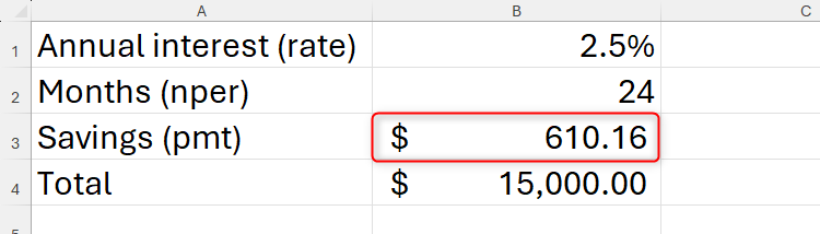
After you click “OK,” Excel runs through several calculation iterations before adjusting the By Changing Cell you referenced earlier. In this case, it tells you that you must save $610.16 per month for two years to reach your goal.

However, at this point, you realize that you can’t afford to save that amount each month. Instead, you decide to carry on putting $400 away each month, and you’ll move house once you’ve reached the $15,000 goal. So, this time, you want Excel to tell you how long that will take.

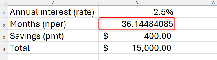
First, manually reset the pmt value in cell B3 to $400. Then, select the cell containing the end value calculation, and click What-If Analysis > Goal Seek in the Data tab.

Again, the set cell is B4, and the end value is still 15000, but the cell that can be changed is the month cell, which is B2.

Finally, click “OK” to reveal that saving $15,000 by paying $400 a month with an interest rate of 2.5% will take just over 36 months.

So, Excel’s Goal Seek tool has helped you work out that if you’re desperate to move house in two years, you’ll need to raise $610.16 per month. On the other hand, if you want to continue paying only £400 a month, you can move house in just over three years.

As well as helping you with your savings, Excel’s Goal Seek tool can help you work out how many products you must sell to reach your target, or what interest rate you need to secure to make a loan affordable.

3Camera Tool for Taking Data Snapshots

Microsoft Excel’s Camera tool allows you to take a snapshot of some data and paste it as an image. What’s more, this image is dynamic, meaning it updates to reflect any changes in the original data.

This tool can be useful if you want to create a dashboard that pulls in data from multiple worksheets in your workbook, and it can also be handy if you’re working with large datasets and want to keep key information in sight. Since the data is duplicated as an image, it sits on top of Excel’s cells without affecting the layout of your spreadsheet.

To do this, click the down arrow on the right-hand side of the ribbon. If you can see “Hide Quick Access Toolbar,” the QAT is already activated. However, if you see “Show Quick Access Toolbar,” click this option to activate it.

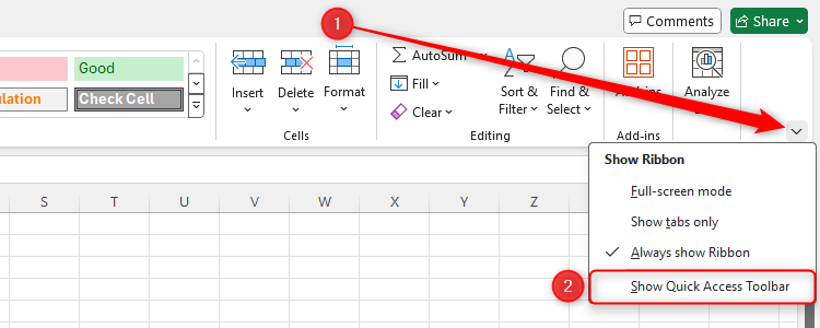
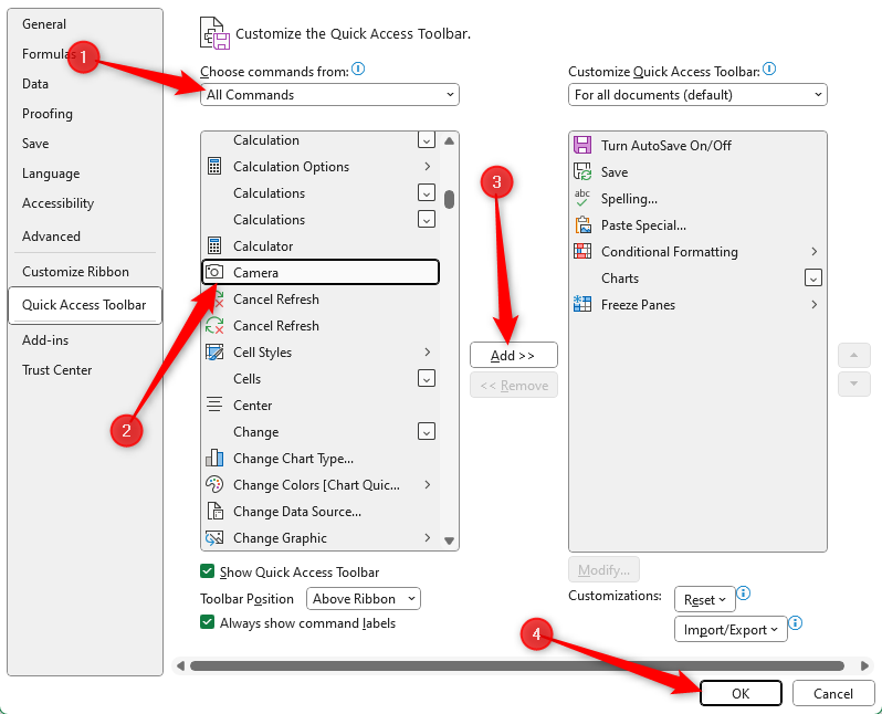
Then, click the down arrow in the QAT at the top of the Excel window, and select “More Commands”.

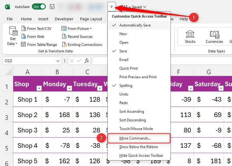
Next, in the Choose Command From drop-down menu, click “All Commands,” and scroll to and select “Camera.” Then, click “Add” to add it to your QAT, and click “OK” to close the dialog box.

Now, the Camera tool is sitting on your QAT, ready to be used.

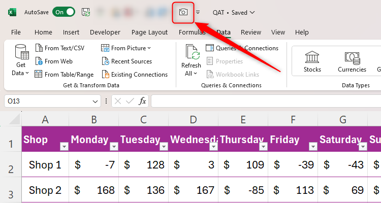
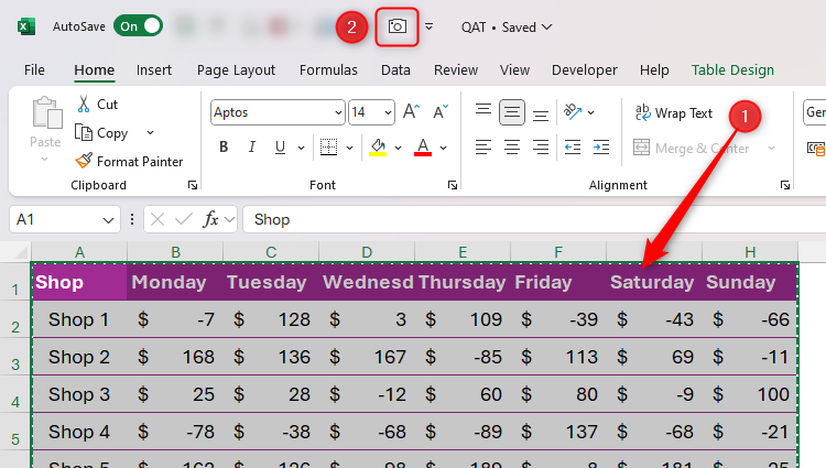
Let’s imagine you need to take a snapshot of some data entered into an Excel table. To do this, select the cells containing that data, and click the “Camera” icon in your QAT.

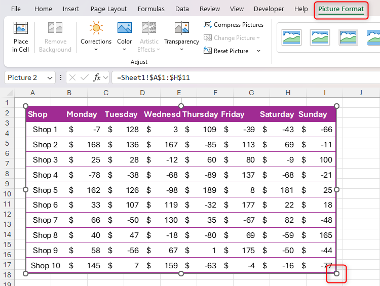
Now, click the cell where you want the image version of this copied data to be duplicated. The Camera tool can work across separate workbooks, but changes to the original data will only be reflected in the pasted image if you’ve signed in to your Microsoft account and activated AutoSave on both files.

Because the data is replicated as an image, you can click and drag the handles to resize the graphic, and you can format the snapshot using the Picture Format tab on the ribbon.

The Camera tool also works on other elements in Excel, like charts and shapes. Simply select the cells behind and around the object, and click the Camera tool in your QAT. Once you’ve pasted the data as an image, crop the image to remove any unwanted space from the edges.

If you’re working on a Microsoft Excel spreadsheet that contains lots of columns, you might be fed up with repeatedly scrolling left and right to read your data. Also, sometimes, certain columns may not always need to be visible.

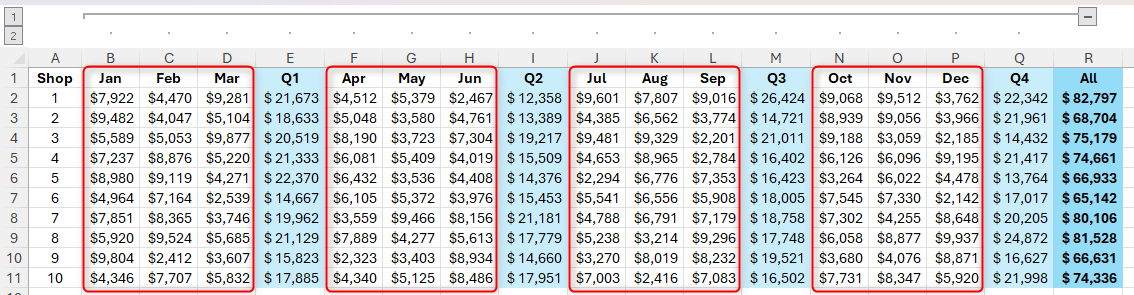
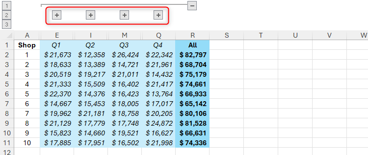
Suppose you have this workbook containing monthly sales figures for various shops, and a yearly total in the rightmost column.

To analyze the annual data and make the figures easier to read, you want to hide columns B to Q, meaning columns A and R will sit next to each other on your worksheet.

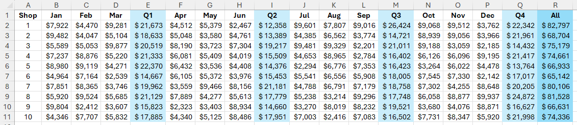
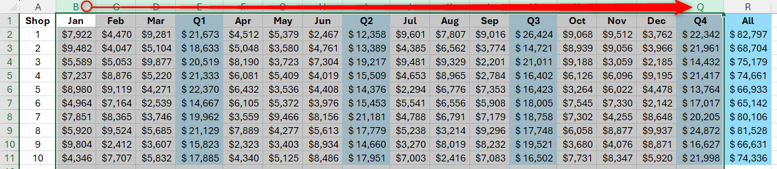
At this point, you might be tempted to select columns B to Q, right-click one of the selected column headers, and click “Hide.” However, it’s easy to forget that these columns are hidden, and the process of unhiding them again is cumbersome. Instead, select columns B to Q by clicking the header for column B and dragging the selection to column Q.

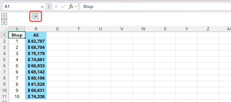
Now, you can click the minus sign or group indicator line above those columns to hide that group.

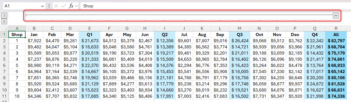
Notice how, when you do, the minus sign turns into a plus sign, which you can click to re-expand that group if you wish.

You can also create subgroups within the main groups, provided each subgroup is separated by a blank or a total column.

Using the same example as above, let’s say you also want to collapse the monthly data, leaving only the quarterly and annual totals visible. This is possible because columns E, I, M, and Q act as barriers between each subgroup.

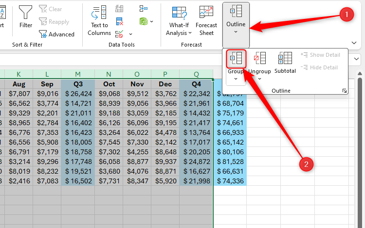
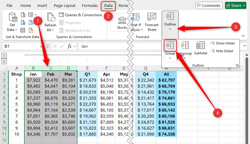
So, to create a subgroup for Q1, select columns B to D, and click “Group” in the Data tab.

Now, as well as having a main group that includes cells B to Q, your spreadsheet also has a subgroup that includes cells B to D.

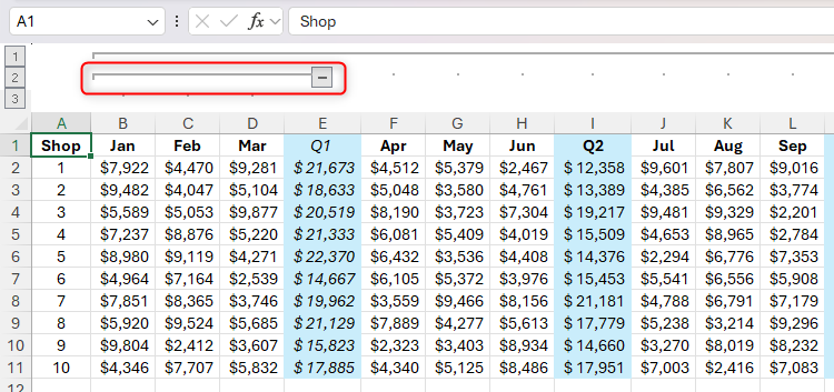
Repeat this process for the remaining quarters until all the subgroups have individual group indicator lines and minus signs. Then, click the four subgroups’ minus signs to display only the quarterly and annual totals, remembering that you can click the plus signs to expand them again.

The Custom Number Format tool is one of my favorite hidden features in Microsoft Excel because it probably saves me the most time.

Every cell in a new spreadsheet has the General number format.

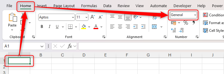
This means that numbers are displayed exactly as they are typed, unless they’re a decimalized number that’s too wide for the cell or a number that starts with zero. However, when you insert a certain type of number—like a date or a percentage—into a cell, Excel recognizes it and updates the number format accordingly.

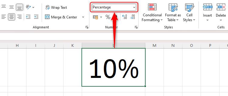
One hidden number format is Custom, which lets you format a cell in a way that isn’t listed in Excel’s standard number formats.

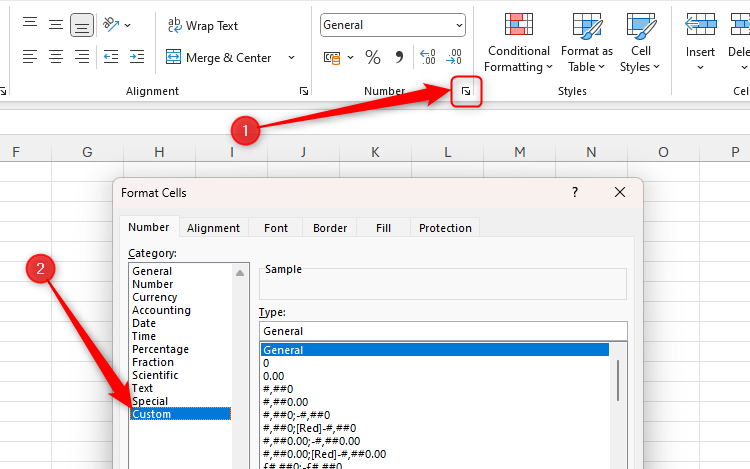
• Select the cell or cells to which you want to apply the formatting you’re about to input, and in the Home tab on the ribbon, click the dialog box launcher in the corner of the Number group.

• Alternatively, press Ctrl+1 to launch the Format Cells dialog box, press Tab to launch the Category menu, and type Cus.

• 

• The information you enter into the Type field depends on the types of data you want to format.

• 

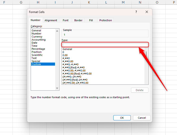
• The first argument you enter formats positive numbers, the second formats negative numbers, the third formats zeros, and the fourth formats text. Notice how semicolons are used to separate the arguments.
• POSITIVE;NEGATIVE;ZERO;TEXT
• One combination you can type into this field is:
• ;;;
• which tells Excel you want the cell to appear blank because you haven’t specified any formatting for any type of data.
• On the other hand, typing:
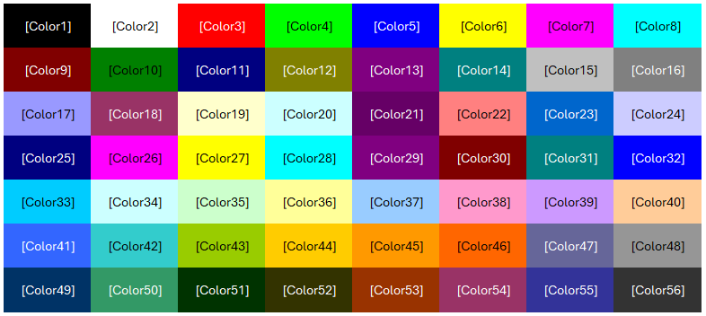
• [Green]#.00;[Red]#.00;[Blue];
• turns positive numbers into a green value with two decimal places, negative numbers into a red value with two decimal places, zeros blue, and produces a blank cell for any text values.

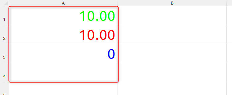
• You may be accustomed to achieving the same outcome using Excel’s Conditional Formatting tool, since this is more prominent on the ribbon than the Custom number format. However, that requires you to input various rules and takes much more time.
• If you want to format values using colors other than black, white, red, green, blue, yellow, magenta, and cyan, type the color code in square parentheses instead of the color name.

• You can also add symbols to a cell’s Custom number format. For example, typing:
• ▲;▼;”=”;
• displays an up arrow instead of positive numbers, a down arrow instead of negative numbers, and an equal sign for zeros.

• If you’re the Windows operating system, press Alt+30 for ▲, and Alt+31 for ▼.

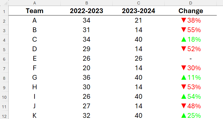
• What’s more, you can combine all the above codes to create neatly formatted cells and improve the visual appeal of your data. For example, typing
• [Green]▲#%;[Red]▼#%;”-“;
• for the Custom format of cells D2 to D12 produces this outcome:

Microsoft Excel’s keyboard shortcuts are also another hidden feature that can truly speed up your workflow. Alongside using the well-known Ctrl+C (copy) and Ctrl+V (paste), take some time to learn some of the lesser-known shortcuts, like F2 for entering a cell’s edit mode and Ctrl+Shift+L for adding filter buttons to the first row of your data.