Situatie
Solutie
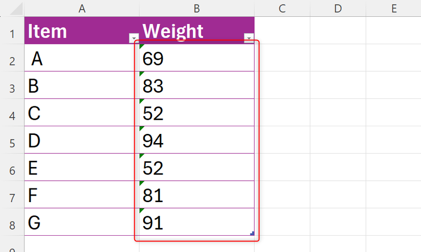
Converting “fake” text to numbers
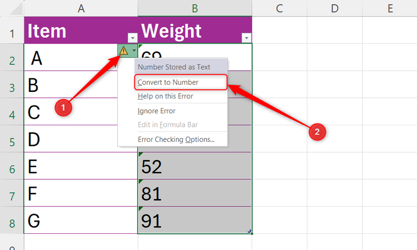
To fix this manually, select the cells, click the exclamation icon, and choose “Convert to Number”
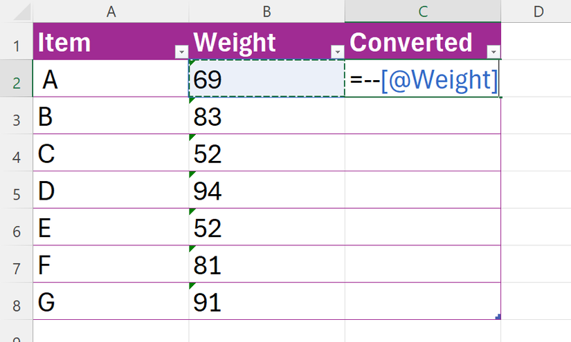
However, if you imported this data and are likely to add more later, the best fix is the double-unary operator (–). In an extra column, type the equal sign (=), add two minus signs (—), and click the first cell containing the “fake numbers.” In my case, I’m applying the fix to the Weight column.
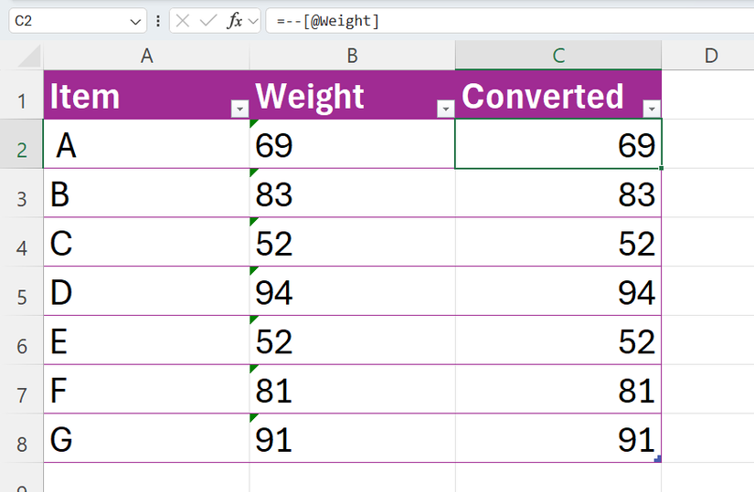
If you’re using an Excel table, when you press Enter, the formula automatically fills down and—most importantly—instantly converts new data you paste into the table.
If the result still looks like text, you need to change the cell’s number format. Select the cells, and in the Number group of the Home tab, choose “General” or “Number.”
The custom number formatting magic
Typing units directly into a cell (like “69 lbs”) turns your data into a text string, breaking any calculations that use this cell.
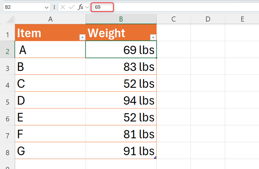
To ensure Excel recognizes the cell as a numerical one while keeping the unit, after deleting the text, select the column, press Ctrl+1, and in the Number tab of the Format Cells dialog, select “Custom.” Then, in the Type field, enter 0 “lbs” (or whichever unit you’re using). Note the double quotes here: they tell Excel to treat the text as a label while leaving the underlying number alone.
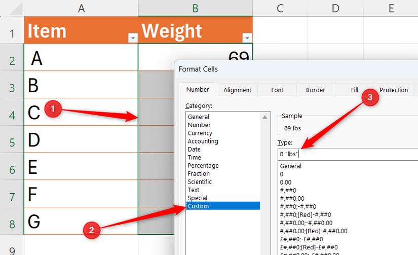
When you click “OK” to close the dialog, you’ll see that even though the cells contain the units, the formula bar displays only the numbers. This confirms that your data is clean and ready to be used in calculations.
If you prefer a cleaner look, simply state the unit in the table header and keep the data underneath as raw numbers.
Surgical extraction: The modern TEXT family
The Text to Columns wizard is a classic, but if your data changes, you have to run the wizard again. If you’re using Excel for Microsoft 365, Excel 2024 or later, or Excel for the web, you should instead use the TEXT family of functions:
| Function | Purpose |
|---|---|
| TEXTBEFORE | Extracts everything before a specific character. |
| TEXTAFTER | Extracts everything after a specific character. |
| TEXTSPLIT | Splits a string into multiple columns or rows. |
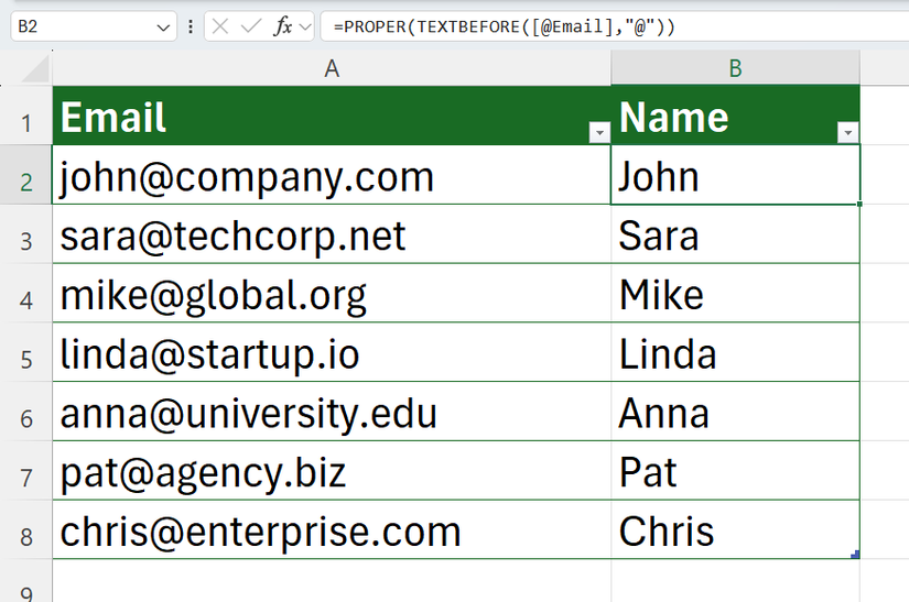
For example, to extract people’s names from these email addresses and capitalize them at the same time, use this formula:
=PROPER(TEXTBEFORE([@Email],"@"))
This finds the “@” and grabs everything to its left. Because it’s a formula, it stays live—update the email or add a new one, and the person’s name updates instantly.
For massive datasets, use Power Query, the dedicated engine that can split, trim, and transform millions of rows of text without slowing down your workbook.
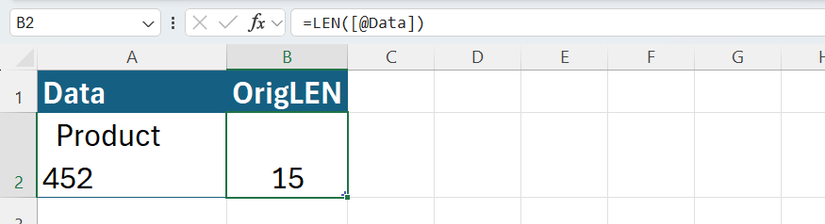
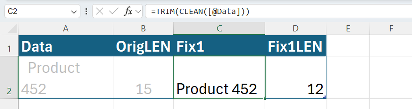
Importing data from external sources into Excel often brings invisible junk, like spaces and non-printing characters. In this example, when I run a LEN character count on the data code imported from the web, I should get 11: seven for the word “Product,” one for the space in the middle, and three for “452.” However, I get 15, meaning there are hidden characters.
The old-school fix is a combination of TRIM (to remove extra spaces) and CLEAN (to strip out non-printing characters):
=TRIM(CLEAN([@Data]))
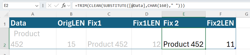
However, this still returns 12, not 11, meaning there’s a ghost character that TRIM is completely blind to.
=TRIM(CLEAN(SUBSTITUTE([@Data],CHAR(160)," ")))
By nesting these, you force Excel to convert the non-breaking spaces—CHAR(160)—into something TRIM can see and strip away. When you run your LEN check again, you’ll hit that perfect 11.
Joining text: Why TEXTJOIN beats the ampersand
The old-school way to combine text in Excel was the ampersand (&):
=[@First]&" "&[@Last]
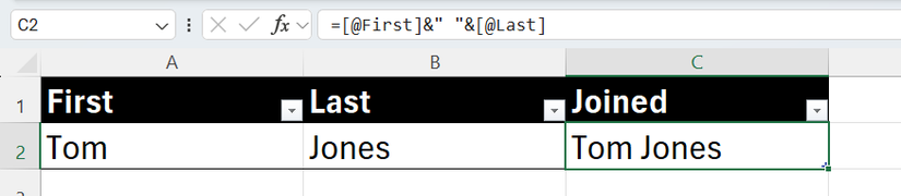
However, if a cell it references is empty, you end up with a string of double-spaces or repeated delimiters.
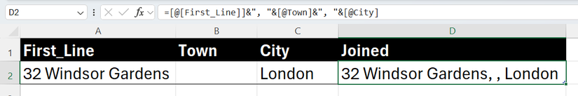
The more robust solution in Excel for Microsoft 365, Excel for the web, or Excel 2019 and later is the TEXTJOIN function. It allows you to set the delimiter once and, crucially, includes a setting to ignore empty cells:
=TEXTJOIN(", ",TRUE,T_Addresses[@[First_Line]:[City]])
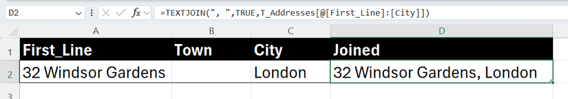
By setting the second argument to TRUE, Excel skips any null values, ensuring your list looks professional regardless of gaps in the data.
For long descriptions or joined strings, click “Wrap Text” in the Home tab to keep your data visible without manually resizing columns. To force a line break, press Alt+Enter.
When a text pattern is too complex to solve with a formula, you can let Excel do the hard work for you. In this example, as soon as I start entering the zip codes from the address, Flash Fill picks up the pattern and offers to complete the column. Just press Tab or Enter to accept the suggestion.
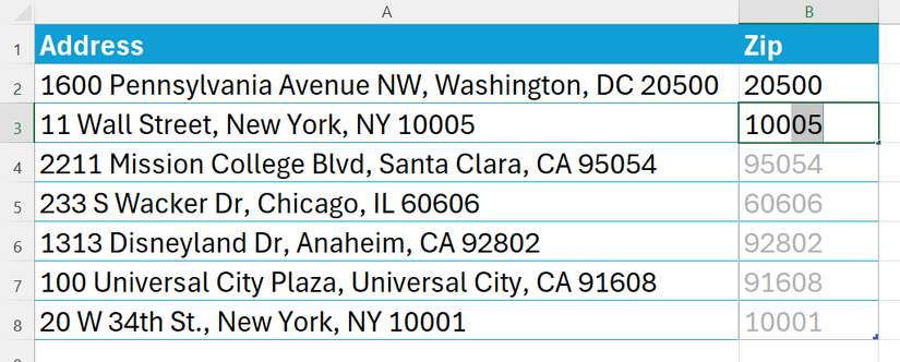
You can also press Ctrl+E to force Excel into this process if the suggestions don’t appear automatically.
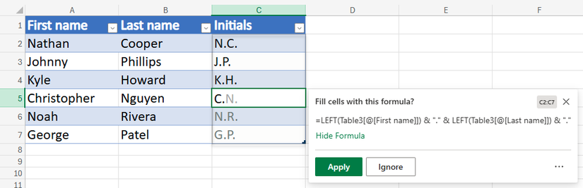
The Formula by Example tool takes this further by actually generating the underlying formula for you. Start typing your pattern, and when Excel suggests a formula, click “Apply.” This is arguably more useful than Flash Fill because the resulting formula reacts to any changes in the original data and works on additional data added to the table.
Leave A Comment?