Stații de lucru

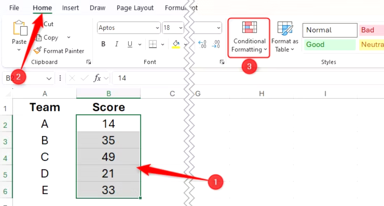
How to creating Bar Charts using the REPT Function in Excel

• Data 06/08/2025
• Autor thomas murarasu
• 0
• 44

Another way to create in-cell bar charts is to use the REPT function, which repeats a specified character a given number of times.

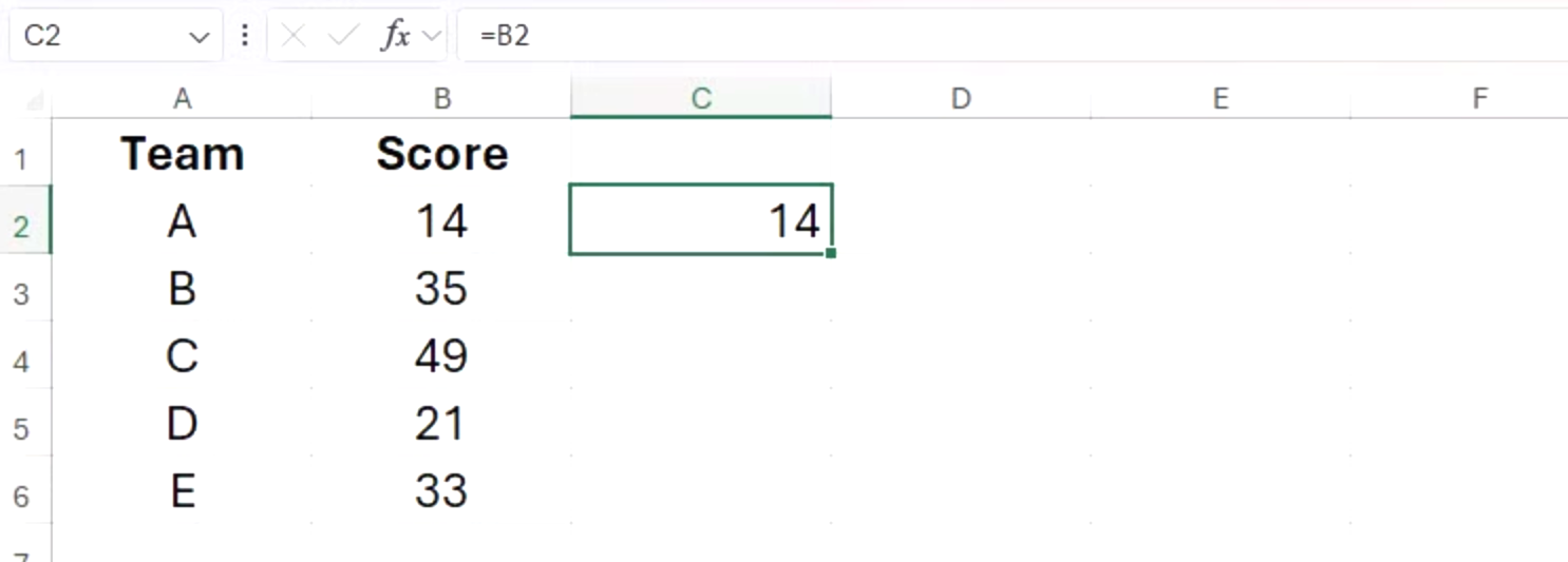
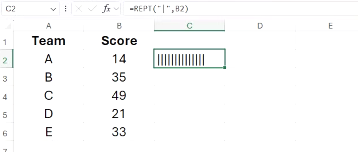
In the cell next to the first value you want to visualize, type:

=REPT("|",x)

and press Ctrl+Enter.

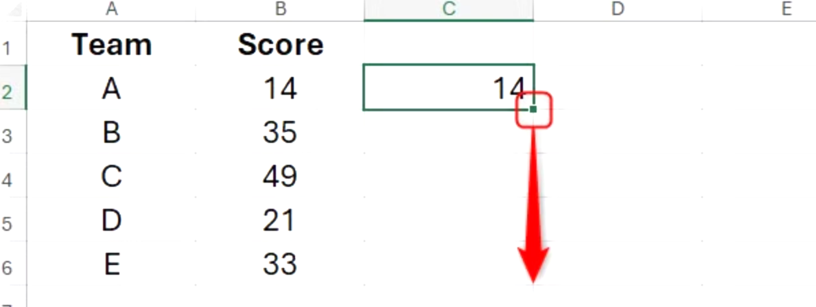
In this formula, “|” is the vertical glyph character (enclosed in double quotes) often accessed by pressing Shift or Fn at the same time as the relevant key, and x is a reference to a cell containing a numerical value. Here, the formula references cell B2 and so returns 14 vertical glyphs.

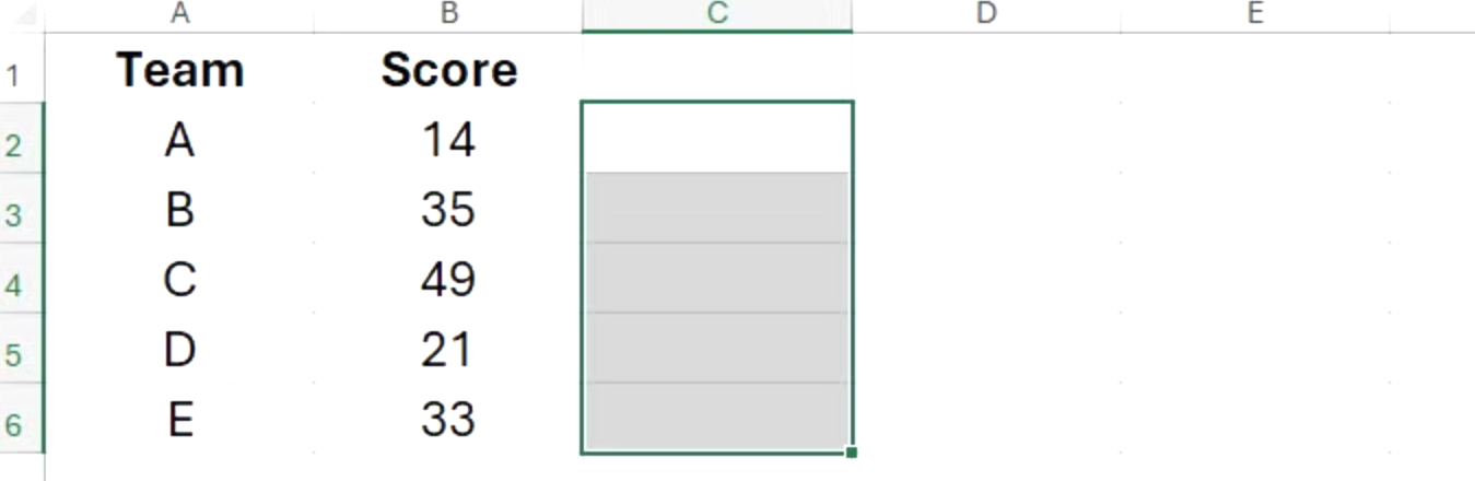
Double-click the fill handle of that cell to repeat the formula down the column.

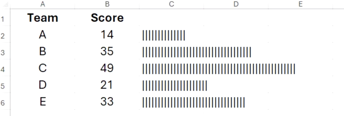
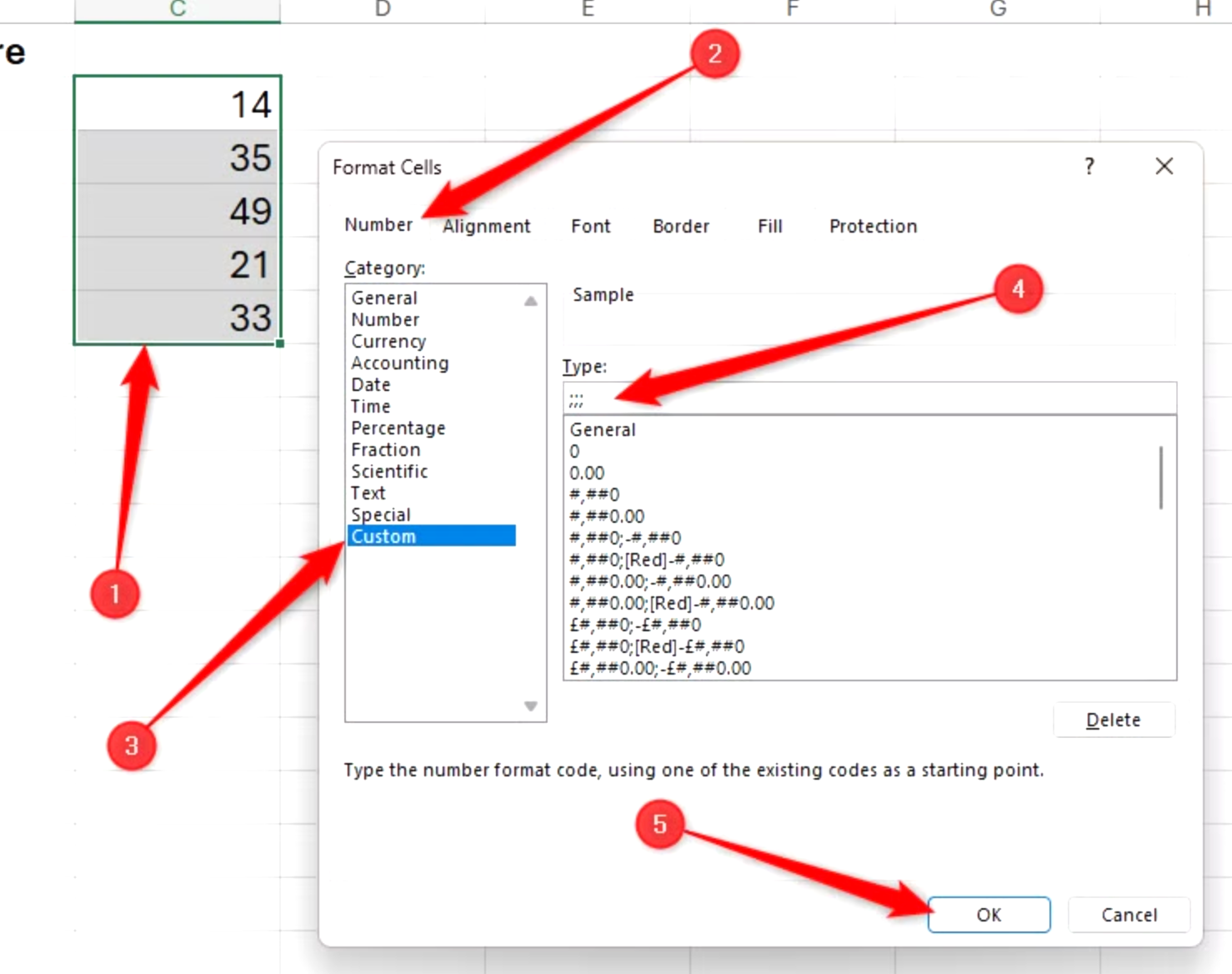
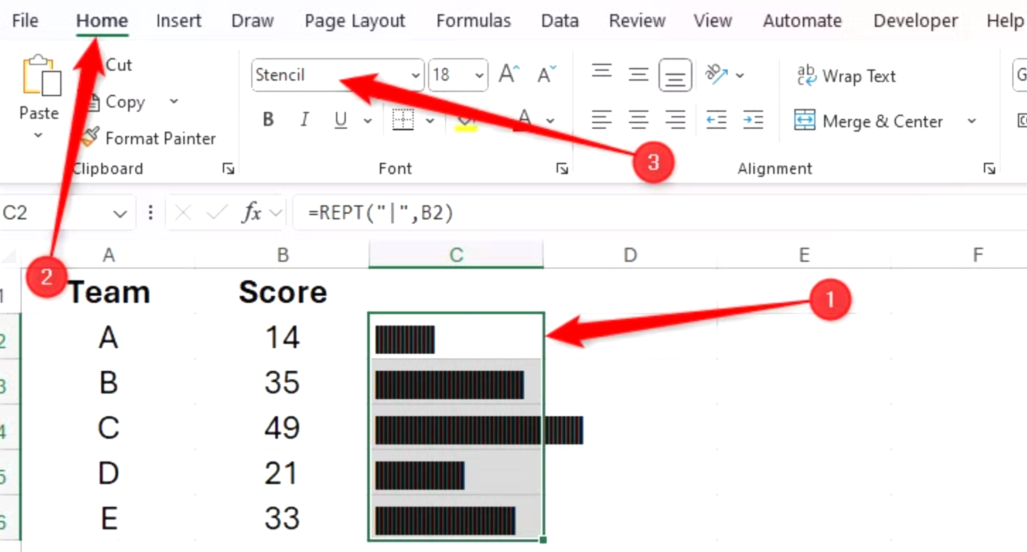
At the moment, the data is visualized as a tally graph, as the default fonts in Excel place small spaces between each character. To fix this, select the relevant cells, and in the Home tab on the ribbon, select a typeface that doesn’t separate characters with a space, like “Stencil” or “Playbill.”

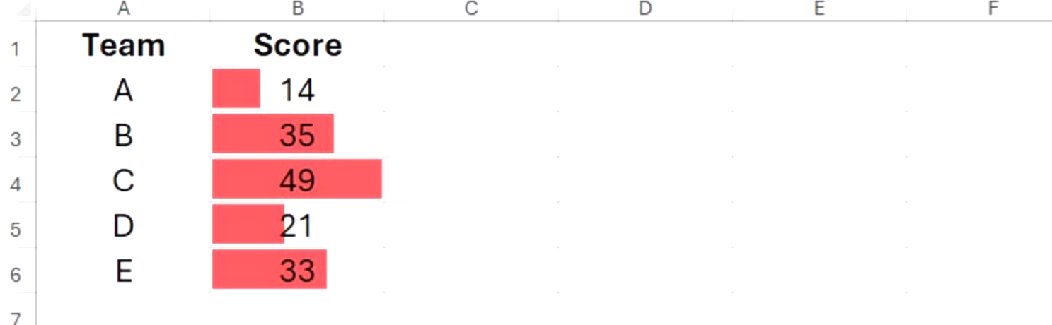
Where data bars adjust to the column width, bar charts created using the REPT function expand or contract dynamically, regardless of the width of the cells they occupy.

How to creating Bar Charts using conditional formatting in Excel

• Data 06/08/2025
• Autor thomas murarasu
• 0
• 37

To create in-cell bar charts using conditional formatting, select the cells containing the values, and in the Home tab on the ribbon, click “Conditional Formatting”

Then, hover over “Data Bars,” and select a fill type.

Now, the cells you selected are partially filled according to their relative values in the dataset. The largest value is represented by a fully filled cell, while only zeros will be completely empty.

What’s more, if the values change, so do the lengths of the data bars.

However, maybe you want the data bars to be next to the cells containing the values. In the screenshot above, that would mean that column B contains the values, and column C contains the data bars. To do this, first, select cell C2, type:

=B2

and press Ctrl+Enter to stay in the same cell.

Now, double-click the fill handle to duplicate the formula down the column.

Next, select the duplicated values you just generated, and press Ctrl+1 to open the Format Cells dialog box. Then, in the Number tab, click “Custom,” type ;;; (three semicolons) into the text field, and click “OK.”

Even though the cells in column C appear empty, they still contain the values you duplicated from column B earlier—they’re just invisible.

Now, apply the conditional formatting data bars to the cells containing the invisible values.