
How to creating Bar Charts using conditional formatting in Excel
To create in-cell bar charts using conditional formatting, select the cells containing the values, and in the Home tab on the ribbon, click “Conditional Formatting”
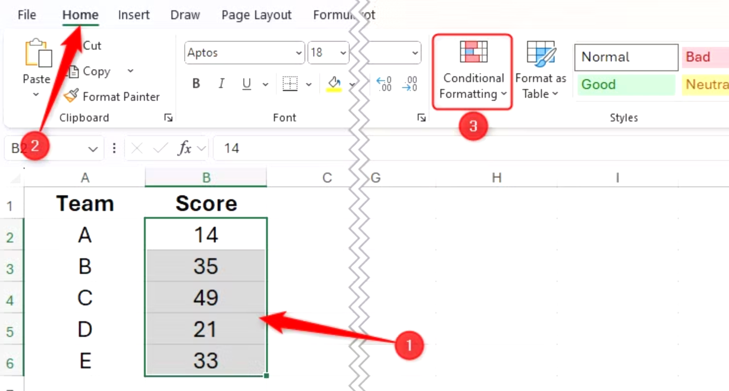
Then, hover over “Data Bars,” and select a fill type.
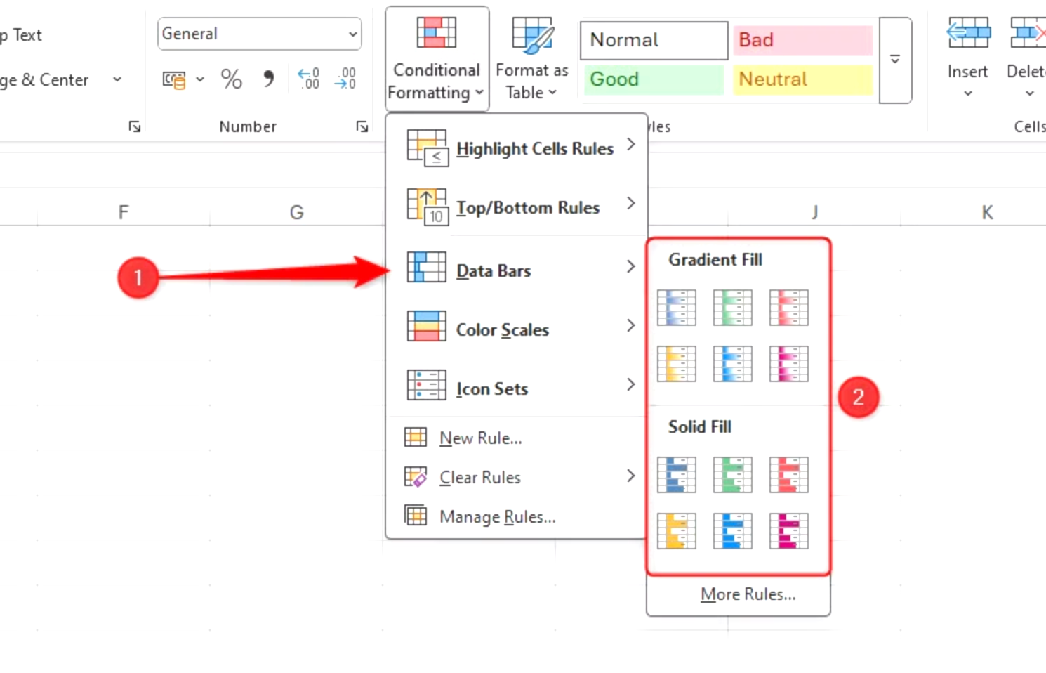
Now, the cells you selected are partially filled according to their relative values in the dataset. The largest value is represented by a fully filled cell, while only zeros will be completely empty.

What’s more, if the values change, so do the lengths of the data bars.
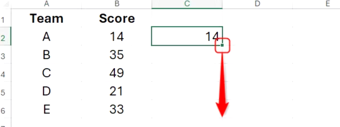
However, maybe you want the data bars to be next to the cells containing the values. In the screenshot above, that would mean that column B contains the values, and column C contains the data bars. To do this, first, select cell C2, type:
=B2
and press Ctrl+Enter to stay in the same cell.

Now, double-click the fill handle to duplicate the formula down the column.
Next, select the duplicated values you just generated, and press Ctrl+1 to open the Format Cells dialog box. Then, in the Number tab, click “Custom,” type ;;; (three semicolons) into the text field, and click “OK.”
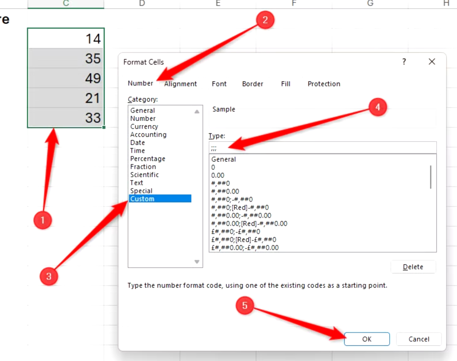
Even though the cells in column C appear empty, they still contain the values you duplicated from column B earlier—they’re just invisible.

Now, apply the conditional formatting data bars to the cells containing the invisible values.
