Creating your own function in Excel using LAMBDA requires you to input two arguments:

=LAMBDA(x,y)

where

• x are the input variables (up to 253), and
• y is the calculation.

The input variables (argument x) can’t clash with cell references or contain periods, and the calculation (argument y) is always the last argument in the LAMBDA function.

Before we look at how LAMBDA can be used in Excel in a real-world scenario, I’ll show you how it works in a basic example.

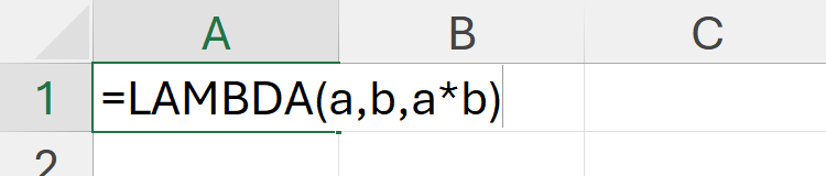
Open a blank Excel workbook, and in cell A1 of Sheet 1, type:

=LAMBDA(a,b,a*b)

but don’t press Enter just yet.

Thinking back to the syntax in the section above, “a,b” is the part of the formula where we identify and name the variables, and “a*b“—the final argument in the formula—is the calculation we want the function to perform when we assign values to those variables. So, for example, if a and b are 4 and 6, respectively, we would expect the calculation to return 24.

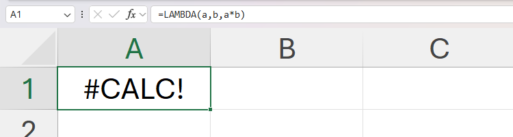
Now, press Enter. At first, this produces a #CALC! error because you haven’t yet assigned any values to the variables.

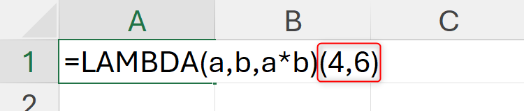
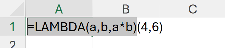
However, you can test that the LAMBDA you have created will work when values are added. To do this, double-click the cell containing the LAMBDA function, and type example variables in parentheses at the end of the existing formula. For example:

=LAMBDA(a,b,a*b)(4,6)

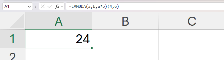
Now, when you press Enter, the cell will display 24, confirming that the LAMBDA formula you created is ready for values to be assigned to the variables.

At this point, you might think that typing =4*6 into a cell and pressing Enter would be much easier, and you’re right. However, the whole purpose of using LAMBDA is to give your calculation a name and apply it to other values whenever needed, which becomes particularly useful when your calculation is more complex. What’s more, if you need to make any changes to the calculation later on, making one minor tweak to your function at its root will impact all relevant calculations, saving you lots of time.

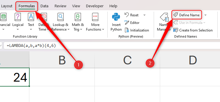
So, to make this happen, double-click the cell containing your LAMBDA function, select the original LAMBDA variables and calculation you created (up to the end of the first set of parentheses), and press Ctrl+C to copy this formula.

Once you’ve copied the formula, press Esc. Then, in the Formulas tab on the ribbon, click “Define Name”

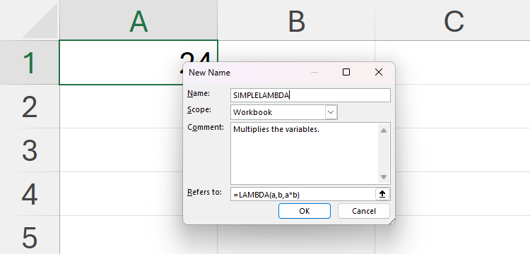
The New Name dialog box that appears is where you will formally define the new function that you can use anywhere within your workbook.

Here’s what each of the fields in this dialog box does and what you need to enter:

This is how your New Name dialog box should look when you’ve filled out all the fields.

When you click “OK,” you’re ready to test this new function elsewhere in your workbook.

Clear the contents of cell A1 by selecting the cell and pressing Delete. Then, in the same cell, type the equal (=) sign, and start typing the name you just gave to your new function. When you see it appear in the list, press the Down Arrow key until your function is highlighted. Notice that the comment you added in the New Name dialog box appears as a tooltip.

Then, press Tab to select and activate this function. This forces Excel to complete the function’s name and open a set of parentheses, ready for you to add the values that represent your variables.

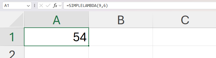
In my example, where I have two variables, I will type:

=SIMPLELAMBDA(9,6)

and press Enter. Remember to close the parentheses!

And hey presto—my new function successfully multiplies 9 by 6 to return 54.

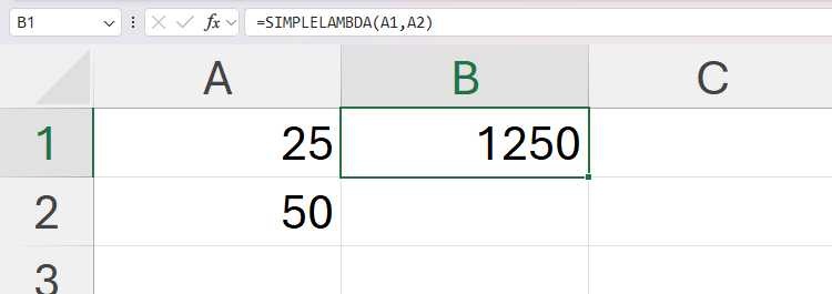
Finally, instead of typing raw data as the variables, try typing cell references. For example, typing:

=SIMPLELAMBDA(A1,A2)

into cell B1 and pressing Enter multiplies the value in cell A1 by the value in cell A2.

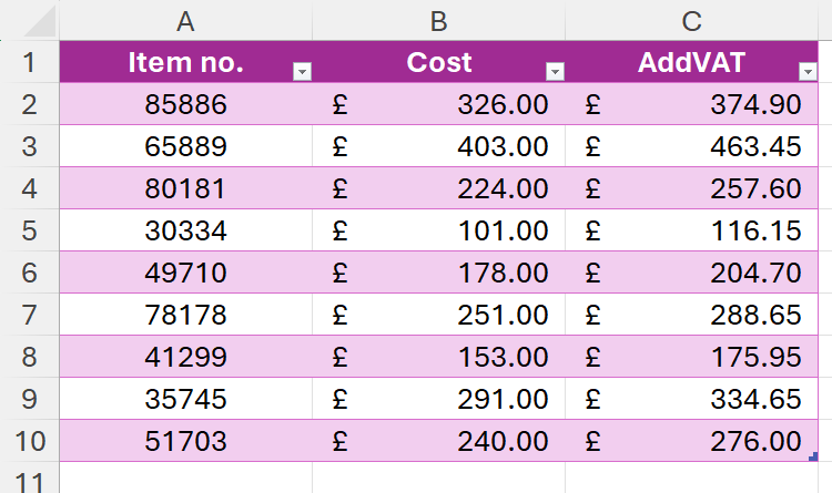
In the UK, VAT is 20%. Let’s assume you want to create a LAMBDA function that adds this value to all costs in your workbook, so that you know the full cost with VAT included.

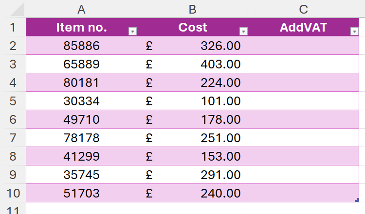
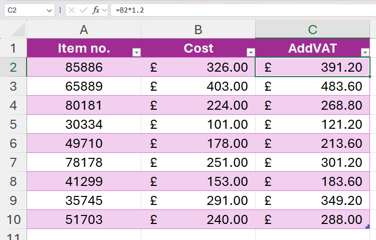
Start by generating the calculation in the first AddVAT cell:

=B2*1.2

and pressing Enter.

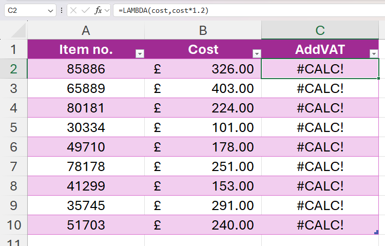
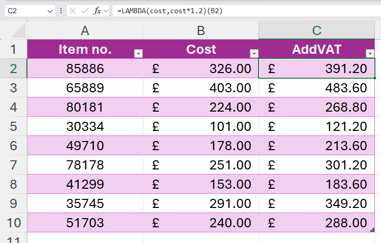
Now, double-click cell C2, add the LAMBDA function, enclose the formula in parentheses, give your variable a name (in this case, you can use cost), and replace the cell reference with this variable in the calculation:

=LAMBDA(cost,cost*1.2)

As with the straightforward example in the section above, this formula alone will return the #CALC! error when you press Enter because you haven’t yet assigned any values to the cost variable.

However, you can test the LAMBDA calculation in cell C2 by adding a temporary variable in the form of a cell reference in parentheses:

=LAMBDA(cost,cost*1.2)(B2)

When you press Enter, you will see that the value in cell B2 and all the other values in column B are successfully multiplied by 1.2 to create the +20% calculation we’re going to automate.

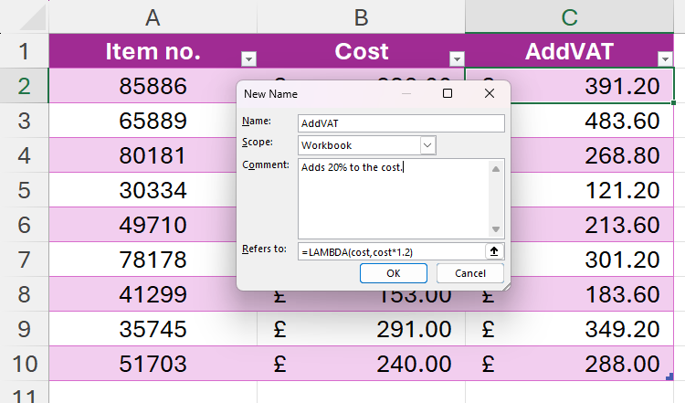
Next, so that you can use this LAMBDA calculation anywhere within your workbook, copy the LAMBDA formula (everything up to the end of the first parentheses), and click “Define Name” in the Formulas tab.

In my example, Excel has automatically populated the Name field in the dialog box with the column header in my table. Once you’ve checked that you’re happy with this name (or chosen a replacement), ensure “Workbook” is selected in the Scope field, add a comment that briefly describes the function, and press Ctrl+V in the Refers To field to paste the LAMBDA function you just copied. Then, click “OK.”

Now, delete all the original data in column C, and type your new AddVAT function into cell C2:

=AddVAT(B2)

When you press Enter, Excel will perform this new calculation, and if you’re using a formatted Excel table, it will apply the calculation to the remaining cells in column C.

Let’s suppose that, in a few years’ time, VAT in the UK is reduced to 15%. The benefit of using LAMBDA is that you don’t have to go through all your calculations and amend them manually. Instead, you only need to adjust the function at its source.

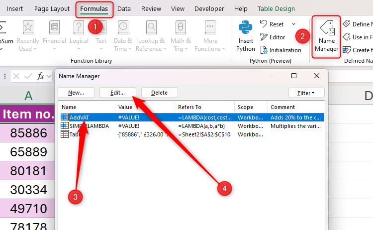
To do this, click “Name Manager” in the Formulas tab on the ribbon, find and select the LAMBDA function you want to adjust (in this case, it’s the “AddVAT” function), and click “Edit”.

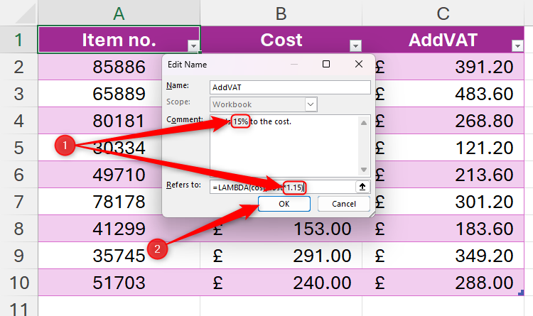
Now, in the Refers To field, change “1.2” to “1.15” to reflect the drop in VAT. Also, cast your eye over the Comments field to see whether you need to adjust the description. Then, click “OK”.